Multi-Stage Analyses and Correlated Uncertainty Propagation

A continuum lattice result is often the output of a directed dependency graph: configurations produce correlators and a scale; correlators produce fitted quantities; separate vertices produce renormalization factors and tuning corrections; all enter a correlated continuum fit. Propagating only the final marginal error from each stage discards shared-input covariance and can count the same variation more than once.

Required background. Estimators, covariance, and resampling define joint propagation, and scale setting supplies a common nuisance input.

Helpful background. Nonperturbative renormalization and step scaling shows a correlated operator-map stage.

Draw the dependency graph first

Local propagation convention and regime. Every reported quantity is a node in one directed acyclic graph whose edges record deterministic transformations or conditional draws. Shared configuration blocks and shared external inputs use aligned outer resample labels; genuinely conditional stochastic estimates use documented inner draws. A marginal error is never treated as independent merely because it was produced by another stage, and linear propagation is used only after checking the relevant nonlinear range.

For every output node, record its parents, whether they share ensembles or external inputs, and the transformation applied. A representative observable is

$$Q_e=Z_e(\mu,a_e)\,a_e^{-d}\, M_e^{\mathrm{bare}}(\boldsymbol\theta_e),$$

followed by a global fit

$$Q_e=Q_\star+c_a(a_e\Lambda)^p+c_Le^{-mL_e}+\cdots.$$

$M_e$, $a_e$, $Z_e$, the tuning variables $\boldsymbol\theta_e$, and sometimes $m$ can share configuration histories and auxiliary fits. Their joint distribution, not a list of marginal standard deviations, is the input.

The chapter figure is a semantic version of this graph.

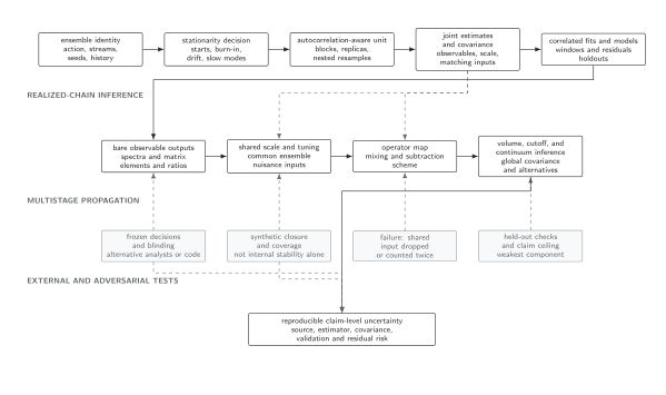
Observable, scale, and operator-map nodes share upstream histories and nuisance inputs. Solid propagation and dashed shared-input arrows must both reach the continuum fit and final uncertainty. The diagram is schematic.

Three valid propagation strategies

Joint model. Fit raw or intermediate data simultaneously with shared nuisance parameters and a block covariance. This exposes correlations directly but can be large and model sensitive.

Aligned nested resampling. Draw outer configuration blocks and shared external inputs, rerun every dependent fit, then draw conditional inner stochastic or calibration inputs. This captures nonlinear transformations but is computationally expensive. The resampling principles underlying this construction are developed by Efron and Tibshirani 1993 and Davison and Hinkley 1997.

Linear propagation. Stack all inputs in $\mathbf x$ with covariance $C_x$ and use

$$C_y=J C_xJ^T, \qquad J_{ij}=\frac{\partial y_i}{\partial x_j}.$$

This is transparent for nearly Gaussian small uncertainties. Check it against resampling when ratios, constraints, or fit boundaries create nonlinearity.

The law of total covariance clarifies nested sources:

$$\operatorname{cov}(Y)= \mathbb E_X[\operatorname{cov}(Y\mid X)] +\operatorname{cov}_X(\mathbb E[Y\mid X]).$$

The first term is conditional stochastic variation; the second is shared outer variation. Adding an independently estimated total error from an inner stage to an outer-resampled error can include the second term twice.

Adversarial failure: a shared scale fluctuation is separated

Let $Q=a^{-d}\widehat Q$. If aligned resamples vary $a$ and $\widehat Q$ jointly, the distribution of $Q$ already contains scale variance and covariance. Adding $d\,\sigma_a/a$ in quadrature afterward double counts it. Conversely, holding $a$ fixed in resamples and never adding its covariance omits the source.

For an exactly checkable $d=1$ fixture, take $z=\pm1$ with equal probability and

$$a(z)=1+0.01z, \qquad \widehat Q(z)=2(1+0.01z).$$

Aligned samples give $Q(z)=\widehat Q(z)/a(z)=2$ identically. If the scale and bare observable labels are shuffled independently, the four possible ratios are $2$, $2$, $2(1.01/0.99)$, and $2(0.99/1.01)$, producing a spurious fractional standard deviation of about $1.41\%$. A pipeline that consumes only the two marginal error bars cannot recover the exact cancellation and must fail this adversary.

One diagnostic is to freeze each node in turn and recompute the final variance. These conditional changes do not generally add to the total when nodes are correlated, but they reveal sensitivity and sign of covariance. Shapley or ordered decompositions may allocate correlated variance, provided the allocation convention is stated and not confused with uniquely identifiable physics.

Interpolation and continuum fits

Interpolating ensembles to common masses or kinematics creates correlated predictions, especially when one interpolation model spans all ensembles. Pass its coefficient covariance into the continuum fit or combine the stages. Do not treat interpolated points as raw independent measurements.

Model alternatives at upstream stages should be propagated coherently. Combining a “renormalization systematic,” “fit-window systematic,” and “continuum systematic” from variations that all move the same data direction can overcount; selecting each component from a different favorable subset can undercount. Use a joint alternative set or explicitly model correlations. Barlow 2002, lecture article explains why a named systematic source must not be converted mechanically into an independent Gaussian error.

Observable-level validation checklist

• Draw the complete dependency graph and label every shared ensemble, calibration datum, nuisance parameter, conditional draw, and covariance handoff.
• Preserve aligned outer resample identifiers across all descendants of a shared input and document every nested inner draw.
• Compare joint fitting, nested resampling, and Jacobian propagation on a linear-Gaussian fixture where all three should agree.
• Recompute the final observable with each node frozen in turn and interpret the change as sensitivity, not as an automatically additive variance component.
• Inject the exact common-factor fixture above and require the pipeline to retain its cancellation and reject independently shuffled labels.
• Repeat interpolation, matching, and continuum alternatives coherently through the final observable and measure end-to-end bias and coverage on synthetic data.

Common pitfalls

Publishing only intermediate error bars. Marginals cannot reconstruct cross-covariance. Preserve samples or full covariance and lineage.

Using independent random resample indices for shared ensembles. That destroys physical correlation among observable, scale, and renormalization estimates.

Adding conditional and marginal errors. Determine which variance is conditioned on which parent before combining.

Learning outcomes

1. Given a multistage lattice result, draw its dependency graph and identify every shared datum, nuisance parameter, conditional source, and covariance handoff needed to reproduce the final observable.
2. Given synthetic aligned and shuffled inputs, compare joint, nested-resampling, and linear propagation and quantitatively expose a dropped, duplicated, or decorrelated uncertainty.

Exercises

1. If $Y=X+\epsilon$ with $\epsilon$ independent of $X$, recover the total-variance formula.

Solution

$\operatorname{var}(Y\mid X)=\operatorname{var}\epsilon$ and $\mathbb E[Y\mid X]=X+\mathbb E\epsilon$, so the two terms give $\operatorname{var}\epsilon+\operatorname{var}X$.

2. Why are two continuum points obtained from one global interpolation correlated?

Solution

They depend on the same fitted interpolation coefficients and often the same scale or tuning data. Variation of those shared parameters moves both predictions coherently.

References

• Barlow, R. (2002). Systematic errors: facts and fictions. In Advanced Statistical Techniques in Particle Physics. arXiv.
• Davison, A. C., and Hinkley, D. V. (1997). Bootstrap Methods and Their Application. Cambridge University Press. DOI.
• Efron, B., and Tibshirani, R. J. (1993). An Introduction to the Bootstrap. Chapman & Hall/CRC. DOI.