Canonical, Fugacity, and Density-of-States Methods

Canonical, fugacity, and density-of-states methods reorganize a finite-density partition function into charge sectors or a one-dimensional oscillatory transform. They can expose physics hidden by direct sampling, but they do not remove cancellation for free: Fourier coefficients may span an exponential dynamic range, reconstructed terms may nearly cancel, and truncation or tail errors are amplified by the condition number of the final sum.

Required background. Anatomy and severity of a sign problem supplies phase and overlap diagnostics. Chemical potential on the Euclidean lattice supplies fugacity and conserved charge.

Helpful background. Fourier series, transforms, and Plancherel theory supplies projection and aliasing. Reweighting, Taylor expansion, and imaginary density supplies the comparison ensemble.

Canonical projection and fugacity reconstruction

Convention and regulator card. At fixed lattice spacing, finite volume, and temperature $T$, let $z=e^{\mu/T}$ and let integer $N$ label the exactly conserved charge in the chosen normalization. Assume the finite regulator gives a finite fugacity range $N_{\min}\le N\le N_{\max}$ or state an explicit tail bound. Imaginary chemical potential is $\mu=iT\phi$.

The grand-canonical partition function decomposes as

$$Z_{\rm GC}(z)=\sum_N Z_Nz^N, \qquad Z_N=\operatorname{Tr}_N e^{-H/T}.$$

On the unit fugacity circle $z=e^{i\phi}$, Fourier orthogonality inverts the relation:

$$Z_N=\frac1{2\pi}\int_{-\pi}^{\pi}d\phi\, e^{-iN\phi}Z_{\rm GC}(z=e^{i\phi}).$$

The period must match the smallest charge unit and any center-twisted periodicity. Using an incorrect period mixes sectors. Canonical finite-density lattice formulations use this projection to separate fixed charge before reconstructing real fugacity Hasenfratz and Toussaint 1992.

For an observable with canonical numerator coefficients $A_N$,

$$\langle O\rangle_\mu =\frac{\sum_NA_Nz^N}{\sum_NZ_Nz^N}.$$

The charge density is

$$\langle N\rangle_\mu =\frac{\sum_NNZ_Nz^N}{\sum_NZ_Nz^N}.$$

These formulas require a common normalization of all sectors. Separate simulations determine $Z_N$ only up to constants unless their relative normalizations are explicitly connected.

With $M$ equally spaced imaginary-μ points, the discrete Fourier transform aliases $N$ with $N+kM$. Exact recovery of a Laurent polynomial spanning $N_{\min},\ldots,N_{\max}$ requires enough points and a convention that distinguishes the full range. Noise breaks exact orthogonality and can make high-$|N|$ coefficients complex or negative even when exact $Z_N$ is nonnegative; symmetry projection may reduce variance, but clipping coefficients biases the reconstruction.

Cancellation and condition numbers

Let $t_N=Z_Nz^N$. A useful reconstruction condition number is

$$\kappa_Z(z)=\frac{\sum_N|t_N|}{\left|\sum_Nt_N\right|}.$$

If coefficient perturbations satisfy $|\delta t_N|\le\epsilon|t_N|$, then

$$\frac{|\delta Z|}{|Z|}\le\kappa_Z\epsilon.$$

Thus $κ_Z$ measures cancellation amplification. For nonnegative exact $Z_N$ and positive real $z$, $κ_Z=1$ at the final fugacity-sum level, yet determining tiny $Z_N$ by Fourier cancellation can itself be exponentially ill-conditioned. Both the projection condition and reconstruction condition must be reported.

If sectors beyond $|N|\le N_{\max}^{\rm keep}$ are omitted, a deterministic denominator bound is

$$|R_Z(z)|\le\sum_{|N|>N_{\max}^{\rm keep}}|Z_N||z|^N.$$

An observable ratio needs bounds on both omitted numerator and denominator tails and a lower bound on the retained denominator. Stability under one truncation change is not a tail bound when coefficients are noisy.

Density of states as an oscillatory transform

Write $S=S_R+iS_I$ and define the generalized density

$$\rho(s)=\int\mathcal D\phi\,e^{-S_R[\phi]} \delta(s-S_I[\phi]).$$

Then

$$Z=\int ds\,\rho(s)e^{-is}.$$

For an observable, define

$$\rho_O(s)=\int\mathcal D\phi\,e^{-S_R[\phi]}O[\phi] \delta(s-S_I[\phi]), \qquad \langle O\rangle=\frac{\int ds\,\rho_O(s)e^{-is}} {\int ds\,\rho(s)e^{-is}}.$$

Algorithms such as LLR estimate local slopes of $\log\rho$ so that densities spanning many orders of magnitude can be reconstructed Langfeld, Lucini, and Rago 2012. The final Fourier integral can still be the difference of much larger contributions. Bin width, slope interpolation, tails, normalization, and arithmetic precision must all be propagated through the oscillatory transform.

If $ρ$ is even, $Z=2\int_0^\infty\rho(s)\cos s\,ds$ is manifestly real but not positive term by term. An approximate fit that is pointwise accurate can give a wrong $Z$ because tiny coherent errors align with $\cos s$. Validate the transform, not merely the density fit.

Exact fugacity fixture

For the one-angle model, set $z=e^\mu$ and

$$Z_1(z)=2\pi\left[(1+h^2)I_0(\beta_0) +hI_1(\beta_0)(z+z^{-1})\right].$$

The only canonical coefficients are

$$Z_0=2\pi(1+h^2)I_0(\beta_0), \qquad Z_{+1}=Z_{-1}=2\pi hI_1(\beta_0).$$

Fourier values at imaginary chemical potential reconstruct them exactly. For $V$ independent copies,

$$Z_V(z)=[Z_1(z)]^V=\sum_{N=-V}^{V}Z_N^{(V)}z^N,$$

and the coefficients are repeated convolutions of the three one-copy coefficients. At least $2V+1$ unaliased Fourier modes are needed for exact discrete reconstruction. The ratio between central and tail coefficients grows rapidly with $V$, creating the intended dynamic-range test at $V=1,4,16,64$.

Three independent checks are available: direct Bessel evaluation of $Z_V$, convolution of exact canonical coefficients, and discrete Fourier projection from imaginary $μ_I=0,\pi/4,\pi/2,3\pi/4$ when the chosen $V$ and symmetry make those four points sufficient only for the low modes being claimed. Four points cannot reconstruct all $2V+1$ coefficients for $V\ge4$; pretending otherwise is the adversarial aliasing failure.

Adversarial failure cases

Stable low-charge reconstruction, wrong density. Central $Z_N$ agree across methods, but real fugacity makes omitted positive-$N$ tails dominate. Bound the tail at the largest $z$ rather than at $z=1$.

Fourier precision floor. High-$N$ coefficients are obtained by subtracting nearly equal complex numbers in double precision. Repeat with increased arithmetic precision and injected-noise studies.

Density fit passes pointwise tests. Residuals for $\log\rho$ are small, but coherent interpolation error changes the oscillatory integral. Compare transforms under alternative bases and against an exact negative control designed at the cancellation scale.

Sector normalizations float independently. Each canonical simulation is precise, yet their unknown relative constants change the fugacity sum. Include an overlap or recursion that fixes all relative normalizations.

The correctness map below groups canonical, fugacity, and density-of-states reconstruction by their shared cancellation problem. Follow the branch to the precision, coefficient-tail, transform, positivity, and exact-fixture tests; formal reconstruction identities do not guarantee numerically resolved sums.

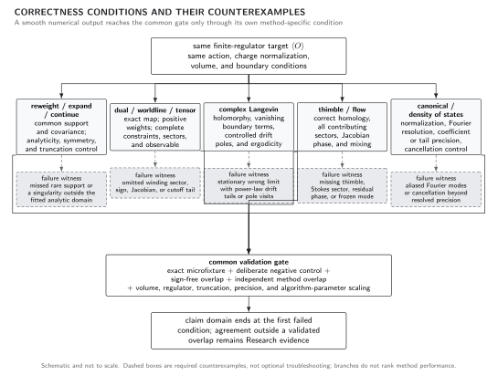
Each reformulation has a different correctness condition and a characteristic counterexample. Apparent numerical convergence is insufficient when overlap is absent, a dual sector or Jacobian is missing, complex-Langevin boundary terms survive, a contributing thimble is omitted, or canonical and density-of-states cancellations exceed resolved precision. The map is schematic and does not rank current algorithms.

Observable-level validation checklist

• State charge units, Fourier period, sector range, grid, arithmetic precision, and normalization convention.
• Test aliasing with injected known modes and compare discrete projection with exact quadrature.
• Propagate the full coefficient covariance through numerator and denominator; report condition numbers.
• Bound canonical and density-of-states tails at every real fugacity used.
• Reconstruct the exact fixture by direct integration, convolution, and imaginary-axis Fourier methods.
• Vary binning, fit basis, truncation, precision, volume, and lattice spacing; keep reach outside the demonstrated range as Research evidence.

Exercises

1. Two-copy canonical coefficients

Compute the five coefficients of $Z_2(z)=[a+b(z+z^{-1})]^2$.

Solution

Expansion gives

$$Z_2=b^2z^2+2abz+(a^2+2b^2)+2abz^{-1}+b^2z^{-2}.$$

Thus $Z_{\pm2}=b^2$, $Z_{\pm1}=2ab$, and $Z_0=a^2+2b^2$. Charge conjugation gives $Z_N=Z_{-N}$.

2. Error amplification

Two terms $t_1=1$ and $t_2=-0.999$ are each known to relative precision $10^{-4}$. Bound the relative error of their sum.

Solution

The sum is $0.001$ and

$$\kappa=\frac{|1|+|{-0.999}|}{|0.001|}=1999.$$

The worst-case relative error is at most $1999\times10^{-4}\simeq0.20$. Four-digit term precision supplies only order-20% control of the cancellation.

Learning outcomes

After working this page, you should be able to:

• Project canonical sectors from imaginary chemical potential, reconstruct a normalized observable, and quantify aliasing and omitted-sector tails.
• Propagate coefficient or density-of-states uncertainty through an oscillatory reconstruction using condition numbers and precision-scaling tests.

Handoff

Cross-method validation and reliability standards combines these reconstruction diagnostics with the correctness tests for reweighting, dual variables, complex Langevin, and contour methods.

References

• Hasenfratz, Anna, and David Toussaint. “Canonical Ensembles and Nonzero Density Quantum Chromodynamics.” Nuclear Physics B 371 (1992): 539–549. doi:10.1016/0550-3213(92)90247-9.
• Langfeld, Kurt, Biagio Lucini, and Antonio Rago. “The Density of States in Gauge Theories.” Physical Review Letters 109 (2012): 111601. doi:10.1103/PhysRevLett.109.111601.