Light-Front Observables and Continuum Validation

A light-front continuum claim is justified only for a named renormalized observable after four classes of tests close together: regulator and basis limits, zero-mode and constraint residuals, current and Poincaré symmetry tests, and an independent benchmark in matched conventions. Agreement of a fitted mass or one current component is insufficient. The strongest claim is set by the weakest unresolved test—especially zero modes, current matching, rotational restoration, or an unseparated cutoff axis.

Required background. Light-Front Regulators, Counterterms, and Symmetry Restoration supplies the cutoff-dependent Hamiltonian and current operator basis. Light-Front Fock Space, Wavefunctions, and Bound-State Equations supplies the state and overlap normalization. Hamiltonian Continuum Limits and Euclidean Cross-Validation supplies the matched-observable comparison with an equal-time or Euclidean regulator.

Helpful background. Complete Lattice Error Budgets supplies correlated uncertainty propagation and coverage tests for a multi-stage extrapolation.

Validation begins with a named observable

Convention and regulator card. Coordinates use $x^\pm=(x^0\pm x^3)/\sqrt2$ and $M^2=2P^+P^- -\mathbf P_\perp^2$. Every result records $(L_-,K,\delta,\Lambda_\perp,N_{\max},b,N_F)$ as applicable, plus boundary, zero-mode, gauge, regulator-field, counterterm, and current prescriptions. Cross-formulation comparisons match the renormalization scheme and scale, state normalization, Fourier transform, momentum transfer, and dimensionless observable. Equal-time periodicity and light-front longitudinal compactification remain distinct finite regulators.

Begin with a vector of target quantities, for example

$$\mathbf O_R =\left( \frac{M_1}{m_R}, F_R(Q_1^2), \frac{\mathcal T_R(s_1,t_1)}{m_R^{\,d_{\mathcal T}}} \right),$$

and mark which entries fix parameters. A quantity used to tune a mass, coupling, current, or symmetry-restoring coefficient is an input. Validation requires other kinematics or observables. If a current is fitted at $Q^2=0$, its slope, another component, or another frame is a natural held-out test.

The criteria on this page are durable method requirements, not an assessment of which light-front program currently reaches a particular precision. Dated capability, comparison, and open-status claims belong to Research.

The validation matrix couples each risk to a falsifier

Minimum evidence for a light-front continuum observable.

Risk	Finite-regulator test	Limit or restoration test	Independent falsifier	Claim if unresolved
Longitudinal resolution and volume	Free dispersion, momentum sum, fixed-box $K$ scan	Separate $K\to\infty$ and $L_-\to\infty$ analyses	Exact integral equation or matched equal-time/Euclidean observable	Finite-$K$, finite-$L_-$ result
Transverse and basis truncation	Residual norm, basis-scale scan, ultraviolet tail	$N_{\max}$ or $\Lambda_\perp$ sequence in more than one basis	Rotation multiplet and frame comparison	Basis-stable estimate only
Fock sectors and counterterms	Sector probabilities and projected equations	Nested sectors with one matching protocol	Held-out mass, scattering point, or current component	Truncation-dependent model result
Zero modes and constraints	Integrated scalar, spinor, and Gauss-law residuals	Boundary/prescription sensitivity and correct limit order	Ward identity, order parameter, topology, or spectrum sensitive to the sector	No vacuum or symmetry claim
Current matching	$F(0)$, charge, and operator-renormalization conditions	Ward identity, component, frame, and angular-condition restoration	A current component or momentum transfer not used in fitting	Matched component at fitted kinematics only
Poincaré symmetry	Dispersion and commutator residuals	Multiplet degeneracy and orientation independence	Same invariant observable in inequivalent frames	No Lorentz-covariant continuum claim
Cross-formulation comparison	Convention round trip and regulator-level anchors	Each formulation removes its own regulators first	Exact, perturbative, Euclidean, or equal-time result with shared inputs exposed	Agreement of finite models, not equivalence of QFTs

The last column is not a penalty; it is the scientifically correct ceiling. An accurate finite-regulator result remains valuable when labeled as such.

The shared map below compresses the matrix into one process relation. Read it from each independent regulator axis through its lost-information obligation, then through matching and held-out tests. The structured regulator table preserves the full row-level alternative.

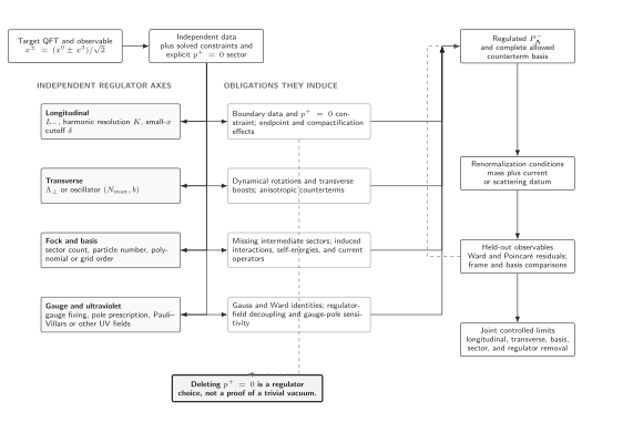
A light-front continuum claim requires the longitudinal, transverse, basis, Fock-sector, gauge, zero-mode, counterterm, current, and symmetry checks to close together. The dashed return path means a failed held-out test revises the regulated operator description rather than being absorbed into the fit; this process diagram is schematic and not to scale.

Currents require normalization and covariance tests

Write the renormalized current as

$$J_R^\mu =Z_JJ_{\mathrm{basis}}^\mu +\sum_a c_a(\boldsymbol\Lambda)\mathcal O_a^\mu.$$

For an elastic charge form factor, test

$$F_R(0)=Q, \qquad q_\mu\langle P'|J_R^\mu|P\rangle=0.$$

The first can be a renormalization condition; the second and nonzero-$Q^2$ behavior must then provide predictions. In a $q^+=0$ frame, $J^+$ often has a simple diagonal Fock overlap, but pair terms, zero modes, or induced current operators can still be required. Truncation can also make different current components disagree even when $F(0)$ is fitted Hiller 2016, § 2.4 and §§ 3.5–3.6, preprint pp. 11–13 and 29–38, PDF.

For a spin-1 state, one common Drell–Yan helicity convention gives the angular condition

$$\Delta_{\mathrm{ang}}(Q^2) =(1+2\eta)I^+_{11} +I^+_{1,-1} -\sqrt{8\eta}\,I^+_{10} -I^+_{00}=0, \qquad \eta=\frac{Q^2}{4M^2}.$$

The phases and normalization of the $I^+_{\lambda'\lambda}$ must be translated when another helicity convention is used. A nonzero $\Delta_{\mathrm{ang}}$ means the four light-front matrix elements cannot be represented by the three physical elastic form factors without orientation dependence. Its role in restoring rotational covariance is derived in Carbonell et al. 1998, §§ 2.1.3 and 3.5, arXiv PDF pp. 13–17 and 51–55.

Current validation is therefore a three-part test: match the operator, enforce its exact identity, and compare redundant extractions. Choosing the extraction that looks smoothest after seeing the data is a model-selection step and must enter the uncertainty.

Poincaré restoration has several observable faces

The invariant mass extracted in a moving frame should satisfy

$$M^2(P^+,\mathbf P_\perp) =2P^+P^-(P^+,\mathbf P_\perp)-\mathbf P_\perp^2$$

independently of external momentum after regulator removal. At finite cutoff, plot the difference between frames rather than averaging it away. In $3+1$ dimensions also test:

• splittings among states expected to form one rotation multiplet;
• commutators involving the dynamical generators $M^{-i}$;
• dependence on the orientation of the null plane;
• dispersion at several longitudinal and transverse momenta; and
• the angular condition or equivalent redundant current relations.

A theory can reproduce a scalar mass while failing spin splittings or current covariance. No one residual is a universal proxy for all Poincaré relations. The front-form generator structure and the dynamical nature of transverse rotations are reviewed in Brodsky, Pauli, and Pinsky 1998, § 2F, arXiv PDF pp. 23–27.

In $1+1$ dimensions there is no transverse rotation. Inventing a “rotational restoration” plot there is not an additional check; use boost/frame, constraint, current, and exact-spectrum tests appropriate to that dimension.

The free scalar provides two common continuum anchors

For a canonically normalized free real scalar in $1+1$ dimensions,

$$\frac{M_1}{m}=1.$$

The Euclidean momentum-space two-point function is

$$G_E(Q^2)=\frac{1}{Q^2+m^2},$$

so the declared spacelike checkpoint is

$$m^2G_E(Q^2=m^2)=\frac12.$$

The one-particle DLCQ mass equals $m$ for every represented nonzero mode, which is an exact convention anchor. It cannot test compactification effects in an interacting state or validate a reconstructed spacelike propagator. A light-front reconstruction must specify how the Minkowski Hamiltonian matrix elements produce the Euclidean-normalized quantity, then vary $K$ and $L_-$ separately.

A cross-formulation calculation should compare these dimensionless quantities. The analytic values $1$ and $1/2$ do not by themselves constitute an executed cross-formulation validation. Equal-time spatial periodicity and light-front longitudinal compactification must each first reproduce their own regulator-level reference.

Multi-axis extrapolation must be identifiable

Let $\epsilon_i$ denote dimensionless cutoff variables, such as $1/K$, $1/N_{\max}$, a small-$x$ cutoff, or an omitted-sector diagnostic. A useful local extrapolation model may take the form

$$O(\boldsymbol\epsilon) =O_*+\sum_i a_i\epsilon_i^{p_i} +\sum_{i<j}a_{ij}\epsilon_i^{p_i}\epsilon_j^{p_j}+\cdots .$$

This is a hypothesis, not a theorem. The design must vary each $\epsilon_i$ while the others are fixed often enough to identify its coefficient. Exponent choices require analytic power counting or comparison among plausible models. Correlated reuse of renormalization inputs, basis data, or exact benchmarks must be retained in the covariance.

Report separately:

• eigensolver, quadrature, and floating-point errors;
• interpolation or extrapolation model uncertainty;
• longitudinal volume and resolution effects;
• transverse, basis-scale, and Fock-sector effects;
• zero-mode and constraint prescription sensitivity;
• parameter and current matching uncertainty; and
• cross-formulation correlations and convention uncertainty.

Quadrature convergence in a wavefunction does not bound a missing current operator. Similarly, agreement between two methods that share the same counterterm input is correlated evidence.

Adversarial failure: every test follows the fit path

Consider a calculation that changes $(K,N_{\max},N_F)$ together, refits the mass and charge at every point, and shows that the fitted mass and $F(0)$ are constant. Both plotted quantities are fixed by construction, and the diagonal cutoff path cannot separate three errors. Even a visually perfect plateau contains no held-out prediction.

The minimum repair is a Cartesian cutoff scan plus a nonzero-$Q^2$ current or second spectral quantity not used in fitting. Add the zero-mode constraint, Ward identity, frame comparison, and—when the dimension permits—rotation test. Until those close, the result is a calibrated finite-truncation model, not a validated continuum observable.

A defensible claim ladder

1. Finite-regulator correctness: exact identities, basis enumeration, matrix residuals, and regulator-level benchmarks pass.
2. Controlled cutoff trend: each relevant axis is independently varied, matching is repeated consistently, and extrapolation alternatives are resolved within the error target.
3. Renormalized observable: current, Ward, zero-mode, and Poincaré tests pass for a held-out dimensionless observable.
4. Cross-formulation validation: an independently regulated calculation reaches the same matched continuum observable with shared inputs and correlations exposed.

Failure at one rung does not invalidate the lower rungs. It prevents claiming the higher one.

The final rung compares formulations only after each has completed its own observable and limit analysis. In the map below, inspect the shared endpoint: no arrow runs directly from a finite Hamiltonian or basis to the continuum claim.

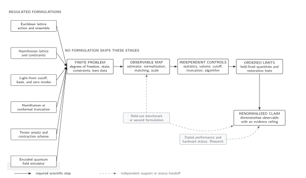
Different regulated formulations can corroborate one QFT observable only after conventions, renormalized quantities, error controls, and limit orders are matched. The schematic does not identify agreement at finite cutoff with continuum equivalence and is not to scale.

Observable-level validation checklist

• Name the target observable, state, scheme, scale, kinematics, and all fitted inputs.
• Record every longitudinal, transverse, basis, sector, zero-mode, gauge, and regulator-field choice.
• Reproduce analytic free or exactly solvable results before interacting extrapolation.
• Evaluate constraint, Ward, Poincaré, frame, orientation, and angular residuals appropriate to the theory and dimension.
• Vary every cutoff independently, compare extrapolation models, and propagate their covariance.
• Reserve at least one mass, current component, momentum transfer, or scattering point that did not influence fitting.
• Match an independent Euclidean, equal-time, perturbative, or exact result only after translating conventions and removing each formulation’s own regulators.
• State the claim ceiling set by any unresolved row of the validation matrix.

You should now be able to (1) build a matrix assigning every light-front cutoff a convergence observable, symmetry test, and independent benchmark, and (2) lower a claim precisely when zero modes, current matching, rotational restoration, or continuum extrapolation remain open. Generic extrapolation and omitted-state certification continue in Convergence, Extrapolation, and Error Certification; matched amplitudes and form-factor definitions continue in Form Factors and Local Operator Insertions; and dated method status remains with Research.

Exercises

Verify the common free benchmark

Compute the two dimensionless free-scalar targets and explain why the exact DLCQ mass does not certify the propagator.

Solution

The one-particle pole has $M_1=m$, hence $M_1/m=1$. At spacelike $Q^2=m^2$,

$$m^2G_E(m^2)=\frac{m^2}{m^2+m^2}=\frac12.$$

DLCQ reproduces $2P^+P^-=m^2$ mode by mode, so it checks the mass-shell normalization. Reconstructing $G_E$ additionally requires a normalized field operator, spectral weights, a continuation or spectral map, and control of $K$, $L_-$, and zero modes. Those ingredients are not tested by the pole location alone.

Use the spin-1 angular condition

At $\eta=1/2$, suppose a convention gives $I^+_{11}=0.8$, $I^+_{1,-1}=0.1$, and $I^+_{10}=0.2$. What value of $I^+_{00}$ satisfies the angular condition? What is the residual if a calculation instead gives $1.28$?

Solution

Here $1+2\eta=2$ and $\sqrt{8\eta}=2$. Therefore

$$I^+_{00}=2(0.8)+0.1-2(0.2)=1.3.$$

If $I^+_{00}=1.28$, then $\Delta_{\mathrm{ang}}=1.6+0.1-0.4-1.28=0.02$. Whether that is acceptable requires a preregistered dimensionless normalization and error target; it cannot be judged from the raw number alone.

References

• Brodsky, Stanley J., Hans-Christian Pauli, and Stephen S. Pinsky. 1998. “Quantum Chromodynamics and Other Field Theories on the Light Cone.” Physics Reports 301: 299–486. DOI. Open PDF.
• Carbonell, Jaume, Bernard Desplanques, Vladimir A. Karmanov, and Jean- François Mathiot. 1998. “Explicitly Covariant Light-Front Dynamics and Relativistic Few-Body Systems.” Physics Reports 300: 215–347. DOI. Open PDF.
• Hiller, John R. 2016. “Nonperturbative Light-Front Hamiltonian Methods.” Progress in Particle and Nuclear Physics 90: 75–124. DOI. Open PDF.
• Karmanov, Vladimir A., Jean-François Mathiot, and Alexander V. Smirnov. 2008. “Systematic Renormalization Scheme in Light-Front Dynamics with Fock Space Truncation.” Physical Review D 77: 085028. DOI. Open PDF.