Timelike Boundaries, Self-Adjoint Extensions, and AdS Boundary Conditions

A timelike boundary can send signals back into the bulk, so the metric and field equation no longer determine evolution. One must choose a boundary condition, equivalently an admissible domain for the spatial operator in static problems. Self-adjointness controls conserved flux and unitary evolution; positivity controls stability. Anti-de Sitter spacetime is the central example because its conformal boundary is timelike.

Required background. Curved Spacetimes, Cauchy Surfaces, and Global Hyperbolicity identifies why a timelike boundary is extra data; Green Operators, Causal Propagators, and State-Dependent Two-Point Functions supplies causal response; Self-Adjointness, Extensions, and Unitary Evolution supplies the operator criterion.

Helpful background. Boundaries and State Preparation supplies the functional-integral perspective; Differential Forms, Integration, and Stokes’ Theorem supplies flux identities.

Boundary forms and self-adjoint domains

On a static spacetime, a scalar equation can often be written

$$\partial_t^2\phi+A\phi=0$$

after choosing the natural weighted spatial Hilbert space. For smooth spatial functions $u$ and $v$, Green’s identity gives

$$\langle u,Av\rangle-\langle Au,v\rangle = \int_{\partial\Sigma} \left( \bar u\,n^iD_iv -(n^iD_i\bar u)\,v \right)\mathrm dS.$$

A self-adjoint domain is a maximal domain on which this boundary form vanishes. Familiar local choices include Dirichlet,

$$u|_{\partial\Sigma}=0,$$

Neumann,

$$n^iD_i u|_{\partial\Sigma}=0,$$

and Robin,

$$(n^iD_i+\kappa)u|_{\partial\Sigma}=0$$

for real $\kappa$ with the boundary orientation stated. More general self-adjoint extensions can be nonlocal along the boundary.

Self-adjointness and positivity answer different questions. A self-adjoint $A$ gives unitary spectral evolution. If $A$ has an eigenvalue $-\lambda^2<0$, then the associated time dependence includes $e^{\lambda t}$, so the dynamics is unstable. A stable ground-state construction requires an extension bounded below, typically $A\ge0$, plus separate treatment of zero modes.

The same boundary form appears in the Klein–Gordon flux. Thus a self-adjoint boundary condition makes the symplectic or Hermitian pairing independent of the Cauchy slice. If the boundary flux is nonzero, the bulk theory is open unless boundary degrees of freedom absorb it.

Scalar asymptotics in anti-de Sitter spacetime

For a scalar of mass $m$ in asymptotically $\mathrm{AdS}_{d+1}$ with radius $\ell$, the two leading radial behaviors are

$$\phi(z,x) \sim z^{\Delta_-}\phi_-(x) +z^{\Delta_+}\phi_+(x),$$

where

$$\Delta_\pm = \frac d2\pm\nu, \qquad \nu = \sqrt{\frac{d^2}{4}+m^2\ell^2}.$$

Reality of $\nu$ gives the Breitenlohner–Freedman lower bound

$$m^2\ell^2\ge-\frac{d^2}{4}.$$

For $0\le\nu<1$, both falloffs lie in the range where a family of positive self-adjoint extensions may be available, subject to the precise geometry and boundary condition. For $\nu\ge1$, the slower falloff is normally excluded by the finite-energy domain, leaving the standard extension. At the endpoints, logarithmic branches require separate analysis. Ishibashi and Wald formulate admissible AdS dynamics in terms of positive self-adjoint extensions of the spatial operator Ishibashi and Wald 2004, §§2–3.

Naming the two coefficients “source” and “response” is a later holographic interpretation. At this stage they label asymptotic data, and a boundary condition specifies an allowed relation between them.

First application: a Robin scalar in static AdS

Choose a Robin relation between the two admissible asymptotic coefficients,

$$\phi_+=\kappa\,\phi_-,$$

with real $\kappa$ in a mass range where both coefficients are normalizable in the relevant energy norm. The associated spatial domain must pass three independent tests:

1. the boundary form vanishes for all pairs in the domain;
2. $A$ is self-adjoint on that domain;
3. the spectrum is nonnegative, apart from zero modes treated explicitly.

If these hold, spectral calculus defines

$$\phi(t) = \cos(A^{1/2}t)\phi_0 +A^{-1/2}\sin(A^{1/2}t)\pi_0,$$

and the Klein–Gordon pairing is conserved. The Green operator and the algebra are those of this particular extension.

For the adversarial test, vary $\kappa$ into a range where an eigenvalue crosses below zero. The boundary condition can remain formally Robin and the operator self-adjoint, yet a mode grows exponentially. Alternatively, choose a boundary relation for which the Klein–Gordon flux does not vanish. Then the bulk pairing depends on the time slice. Either failure blocks a stable closed-system quantization.

Boundary conditions can also change causality at the global level: reflected singularities return from the boundary. A bulk two-point function must have the singularities appropriate to the selected boundary problem, not merely the local Hadamard form before the first reflection.

Construction and failure maps

Read the construction map with the boundary condition included in the first two boxes. It helps determine the Green-hyperbolic boundary problem and therefore the solution space and algebra before a state is chosen.

An AdS boundary condition is part of the dynamical input, not a later state choice; the construction map is schematic and not to scale.

In the failure map, inspect both boundary flux and self-adjointness. Positivity is an additional page-specific test: a self-adjoint extension with a negative mode is not a stable vacuum problem.

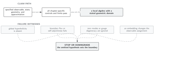
Stable closed evolution requires a flux-compatible self-adjoint domain with controlled lower spectrum; otherwise the claim stops or is downgraded to an open or unstable system. Schematic and not to scale.

The chapter-level comparison is under Domain and failure conditions. This page additionally requires the boundary orientation, operator domain, energy norm, lower spectral bound, and treatment of endpoint or zero-mode cases.

Check your understanding

Why is self-adjointness alone insufficient for a ground state?

Solution

A self-adjoint operator can have negative spectrum. If $Au=-\lambda^2u$, then the mode equation is $\ddot q-\lambda^2q=0$ and has exponentially growing solutions. A stable oscillator ground state requires a suitable nonnegative extension, not merely real spectrum and unitary functional calculus.

AdS boundary correlators and source/response interpretations belong to Volume XV. Boundary algebra theorems and non-globally-hyperbolic extensions remain in Volume XVI.

References

• Akihiro Ishibashi and Robert M. Wald, “Dynamics in Non-Globally-Hyperbolic Static Spacetimes II: General Analysis of Prescriptions for Dynamics,” Classical and Quantum Gravity 20 (2003), 3815–3826, DOI, arXiv:gr-qc/0305012.
• Akihiro Ishibashi and Robert M. Wald, “Dynamics in Non-Globally-Hyperbolic Static Spacetimes III: Anti-de Sitter Spacetime,” Classical and Quantum Gravity 21 (2004), 2981–3014, DOI, arXiv:hep-th/0402184.
• Claude M. Warnick, “The Massive Wave Equation in Asymptotically AdS Spacetimes,” Communications in Mathematical Physics 321 (2013), 85–111, DOI, arXiv:1202.3445.