Background Splitting and Perturbative Agreement

A perturbative calculation begins by choosing a solvable quadratic action, but that choice is not physical. A mass shift, background potential, or metric perturbation may be included in the free operator or treated as an interaction. Perturbative agreement requires the two descriptions to match after propagators, Wick ordering, time-ordered products, counterterms, and states are transported consistently.

Required background. Relative Cauchy evolution and background response explains how observables respond to background changes, and local covariant renormalization restricts the comparison map.

Helpful background. Background-field Yang–Mills gives the gauge-theory analogue, while observable and off-shell matching clarifies which quantities must agree.

One theory, two quadratic decompositions

Write the same action as

$$S=S_0+Q+V=S_1+V, \qquad S_1=S_0+Q,$$

where $Q$ is a compactly supported or otherwise controlled quadratic functional. The first description uses the free operator $P_0$ and treats $Q+V$ perturbatively; the second uses $P_1=P_0+q$ and treats only $V$ perturbatively.

At the classical level, a retarded Møller map identifies solutions and observables of the two quadratic theories. At the quantum level, changing the two-point function changes the star product and Wick ordering. Because two Hadamard parametrices differ by a smooth kernel after their singular structures are matched, an exponential contraction map transports the free algebras. Renormalized time ordering adds a finite local correction. Perturbative agreement is the normalization condition that the exact quadratic transport and the perturbative treatment of $Q$ define the same interacting observable under this composite map.

For scalar quadratic interactions without derivatives, this agreement and its extension to a quadratic part of a general interaction are established by Drago, Hack, and Pinamonti (2017, Theorems 3.2 and 4.1). Metric variations require the stronger time-ordered-product identities used by Hollands and Wald (2005, §§ 4–5).

The construction map shows which objects must be transported when the split changes: propagators and time-ordered products at the left, then local counterterms and identities before the interacting observable at the right. Moving only a parameter skips most of this path.

Perturbative agreement spans the full controlled construction. The map is schematic and not to scale; the exact quadratic and perturbative descriptions agree only after every intermediate structure is identified.

The failure map names surviving split dependence as a direct witness. It should be tested only after the state and finite local map have been transformed; otherwise the apparent failure is manufactured by comparing inequivalent inputs.

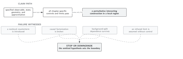
Claim boundary for perturbative agreement. This schematic, not-to-scale map licenses split independence only after propagator, state, operator, and counterterm maps have all passed.

Application: moving a mass term

Take

$$P_0=\Box+m_0^2+\xi R, \qquad q=\delta m^2, \qquad P_1=P_0+\delta m^2.$$

The second free Feynman propagator obeys the resolvent expansion

$$G_{F,1} =G_{F,0}-G_{F,0}\,\delta m^2\,G_{F,0} +G_{F,0}\,\delta m^2\,G_{F,0}\,\delta m^2\,G_{F,0}-\cdots,$$

where products denote covariant integrations. This is exactly the series generated by insertions of

$$Q=-\frac12\int d\mu_g\,\delta m^2\phi^2$$

in the $P_0$ theory, including the signs fixed by the action convention. Thus separated-point two-point functions agree order by order before renormalized coincidences are taken.

Coincidence limits require more. The Wick square defined using $P_1$ has a different Hadamard parametrix from the one defined using $P_0$. Their finite difference contains local terms proportional to $\delta m^2$ and, at higher orders or with other quadratic changes, curvature polynomials. Denote the finite local transport by $Z_Q$. Then the comparison of an observable $F$ has the structure

$$R^{(1)}_V(F) =\beta_Q\!\left(R^{(0)}_{Q+Z_Q(V)}(Z_QF)\right),$$

where $\beta_Q$ is the free quantum identification. The displayed equation indicates the required maps rather than defining a new exact nonperturbative equality: every term is a formal series, and the equality holds through the verified perturbative order.

For a two-point benchmark through first order in $\delta m^2$ and $\lambda$, agreement requires:

1. the propagator insertion $-G_{F,0}\delta m^2G_{F,0}$;
2. the finite change of Wick ordering and composite insertions;
3. the transformed mass, $R\phi^2$, and vacuum counterterms;
4. transport of the Hadamard state, rather than reuse of an unrelated numerical covariance.

After these transformations, smeared correlators in the common local region agree up to $O((\delta m^2)^2,\lambda\delta m^2,\lambda^2)$ if only first-order terms were retained.

Adversarial test: freezing the state and counterterms

Change $P_0$ to $P_1$ but evaluate both descriptions with the same mode coefficients and the same finite normal-ordering constants. The object called “the same state” will generally fail to be a bisolution of both operators. Even if one manually projects it to a state, its smooth two-point part has not been transported by $\beta_Q$. The two tadpoles then differ by a smooth state term and by local $\delta m^2$ and curvature terms.

If the counterterms are also left unchanged, the second description uses renormalization conditions tied to the first free operator. A residual split dependence appears in the two-point function. This is not evidence that the physical theory knows the split; it shows that the comparison omitted part of the map. The strongest surviving statement is an off-shell comparison between two differently normalized perturbative descriptions.

Domain and failure conditions

The common domain and failure-conditions table supplies the chapter context. A controlled quadratic functional, hyperbolic operators for both splits, compatible Hadamard data, and a finite local comparison map license equality of local formal observables through the declared perturbative order. The decisive checks are the separated-point resolvent identity and agreement of renormalized coincidences after state and counterterm transport. Residual dependence after all maps are applied invalidates split independence; dependence before that transport supports only two differently normalized descriptions and cannot be handed to the stress-tensor Ward identity as a physical discrepancy.

Checks and limitations

• Verify the resolvent identity at separated points before diagnosing a renormalization mismatch.
• Transport the state or compare algebraic observables before applying states.
• Match finite counterterms and composite operators, not just bare parameters.
• A large or sign-changing quadratic shift can destroy hyperbolicity or positivity assumptions used to choose a reference state; perturbative agreement is local/formal and does not cure that spectral problem.
• For gauge or metric splits, impose the corresponding BRST or diffeomorphism identities as well as the scalar-type agreement condition.

Exercise

Differentiate the identity $(P_0+s q)G_s=1$ at $s=0$ and recover the first resolvent insertion.

Solution

Differentiation gives $qG_0+P_0\dot G_0=0$. Multiplying by $G_0$ on the left, with the same Green-function boundary prescription, yields

$$\dot G_0=-G_0qG_0.$$

Hence $G_s=G_0-sG_0qG_0+O(s^2)$, which is the first perturbative insertion of the quadratic interaction.

Handoff

Metric perturbations are a particularly consequential background split. Their response defines the interacting stress tensor, so perturbative agreement must be combined with the diffeomorphism Ward identity and its contact terms.

References

• Drago, Nicolò, Thomas-Paul Hack, and Nicola Pinamonti. “The Generalised Principle of Perturbative Agreement and the Thermal Mass.” Annales Henri Poincaré 18 (2017): 807–868. doi:10.1007/s00023-016-0521-6.
• Hollands, Stefan, and Robert M. Wald. “Conservation of the Stress Tensor in Perturbative Interacting Quantum Field Theory in Curved Spacetimes.” Reviews in Mathematical Physics 17 (2005): 227–312. doi:10.1142/S0129055X05002340.