

QEI Sampling, State Domains, and Scheme Dependence
The numerical strength of a QEI depends on the sampling profile, but a meaningful comparison holds fixed a physical duration, normalization, worldline, observable, state class, and finite renormalization prescription. Comparing a Gaussian standard deviation with a compact sampler’s support radius manufactures a discrepancy before curvature or acceleration has entered. This page defines a reproducible comparison in terms of proper-time moments.
Required background. Curved-spacetime QEIs supplies the bound; test functions and distributions supplies smooth support; and adiabatic, DeWitt–Schwinger, and dimensional schemes supplies stress-scheme translation.
Helpful background. States of low energy gives a variational use of sampling, while null-smeared stress observables shows why timelike and null support must remain distinct.
Normalized sampler data
Section titled “Normalized sampler data”Let be real and smooth along a proper-time parametrized worldline. Fix
The flat four-dimensional massless-scalar QEI is
For samplers with the same , the dimensionless shape coefficient
isolates genuine profile dependence. It does not isolate curvature or acceleration unless those are also held fixed.
Compare two families. A Gaussian profile normalized in is
When the theorem is stated only for , use a Gaussian-like compact approximation and demonstrate convergence as grows. A strictly compact bump can be written
with and chosen numerically so that its norm and match the Gaussian. The characteristic functions here only describe the piecewise definition; every derivative vanishes at , so .
The structure map identifies the sampler as theorem data, not presentation detail. Scheme, curve, and state choices remain fixed while only is compared.

Controlled sampler comparison. The map is schematic and not to scale; matching the rms duration removes a width-convention artifact, leaving profile, curvature, and acceleration effects as separately varied quantities.
Inertial and accelerated worldlines
Section titled “Inertial and accelerated worldlines”On an inertial Minkowski worldline the profile enters through . On a uniformly accelerated worldline with proper acceleration , stationary-worldline bounds acquire additional spectral terms. At short duration,
where coefficients and even the convenient representation depend on field and theorem. The correct comparison uses the same , not the same coordinate acceleration. Exact stationary-worldline QEIs and their asymptotics are developed by Fewster and Thompson (Fewster and Thompson 2023, §§ 3–5).
In curved spacetime add independent ratios such as
A profile that has longer tails can sample a region with materially different curvature even at the same rms width. Report the maximum geometric ratios over the actual support or a controlled tail estimate.
Scheme and state comparisons
Section titled “Scheme and state comparisons”If
then the sampled energy and absolute lower bound both shift by
Translating only the data and not the bound creates false scheme dependence. A difference QEI also carries its reference state; changing that state changes both sides and is not a regulator test.
The adversarial comparison calls the Gaussian width its full width at half maximum, calls the compact profile’s width, and sets those unequal notions to the same number. Recomputing exposes the mismatch. Only after rescaling both profiles to the same rms duration may the remaining difference be attributed to shape.
The failure map also catches a hidden state change: minimizing the sampled energy separately for each profile compares different states unless that is the declared variational question.
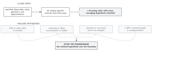
Failure conditions for QEI profile comparisons. The diagram is schematic and not to scale; matched rms duration, curve, state problem, and scheme are required before a change in the bound can be assigned to sampler shape.
Domain and failure conditions
Section titled “Domain and failure conditions”See the chapter domain and failure-conditions table. The comparison assumes smooth proper-time samplers, a free field in the QEI’s Hadamard state class, and fixed curve and stress prescription. Gaussian limits require a convergence argument when the theorem assumes compact support. Long tails, boundaries, nonstationary acceleration, or unmatched reference states require a new bound.
Exercise
Section titled “Exercise”Show that is unchanged when is rescaled to .
Solution
The rms duration scales as , while
Their product is therefore invariant.
References
Section titled “References”- Fewster, C. J., and S. P. Eveson. “Bounds on Negative Energy Densities in Flat Spacetime.” Physical Review D 58 (1998): 084010. DOI.
- Fewster, C. J., and C. J. Smith. “Absolute Quantum Energy Inequalities in Curved Spacetime.” Annales Henri Poincaré 9 (2008): 425–455. DOI.
- Fewster, C. J., and C. J. Thompson. “Quantum Energy Inequalities along Stationary Worldlines.” Classical and Quantum Gravity 40 (2023): 175008. DOI.
Original QFT.org content:CC BY 4.0, unless an item supplies different terms. Third-party material retains its own terms.