Higher Cumulants and Non-Gaussian Noise

The noise kernel fixes only the second connected stress moment. A non-Gaussian matter state, a quadratic stress operator even in a Gaussian field state, or a tail-sensitive metric statistic can require the full connected hierarchy. Higher pure-difference vertices of the influence functional may sometimes be represented by non-Gaussian stochastic cumulants, but a positive joint classical measure is not guaranteed for multitime noncommuting quantum observables.

Required background. Influence Functionals, Dissipation, and Noise supplies the closed-time-path expansion; The Stress-Tensor Noise Kernel fixes the second cumulant; and Connected Correlators and Cumulants fixes connected subtraction.

Helpful background. Characteristic Functions, Cumulants, and Generating Functionals supplies the probability criterion, while Multiplicative, Colored, and Conserved Noise treats generalized stochastic sources.

The stress cumulant hierarchy

For one real smeared stress observable

$$X=\hat t(f), \qquad \langle X\rangle=0,$$

define its characteristic function and cumulants by

$$\chi_f(s)=\left\langle e^{isX}\right\rangle, \qquad \log\chi_f(s)= \sum_{n=2}^{\infty}\frac{(is)^n}{n!}\kappa_n[f].$$

Thus $\kappa_2[f]=N(f,f)$ and $\kappa_3[f]=\langle X^3\rangle$ for a centered single observable. For several spacetime smearings, the corresponding quantum generating functional depends on ordering. The pure $J_\Delta^n$ vertices select fully symmetrized connected stress products, whereas vertices involving both $J_c$ and $J_\Delta$ encode nonlinear response and nested commutators. Replacing all of them by moments of one classical source would discard that distinction.

A proposed classical non-Gaussian source $\xi$ has

$$\mathbb E\exp\!\left(i\xi(f)\right) =\exp\!\left[ \sum_{n=2}^{\infty}\frac{i^n}{n!} \kappa_n[f,\ldots,f] \right].$$

This functional must be continuous, normalized, and of positive type on the chosen real test-function space. Positivity of $\kappa_2$ alone is necessary but not sufficient. Truncating the logarithm after an odd order generally does not define a positive probability law for arbitrary source strength; a cumulant expansion is often asymptotic or perturbative rather than an exact sampling prescription.

The structure map places higher cumulants after the Gaussian large-N comparison. Inspect the new branch: it changes selected higher symmetrized statistics and does not retroactively supply operator ordering.

The Gaussian noise kernel is the second rung of a correlation hierarchy; extending it requires both renormalized higher stress products and a check that the requested stochastic representation exists. The map is schematic and not to scale.

First application: a non-Gaussian scalar-mode state

Select one ultrastatic scalar mode and a smooth stress sampler whose normal-ordered contribution is $\lambda\hat n$. Consider the diagonal state

$$\rho_p=(1-p)|0\rangle\langle0| +p|1\rangle\langle1|, \qquad 0<p<1,$$

and center the observable,

$$X=\lambda(\hat n-p).$$

Its first three connected moments follow directly from the Bernoulli distribution:

$$\begin{aligned} \kappa_1[X]&=0,\\ \kappa_2[X]&=\lambda^2p(1-p),\\ \kappa_3[X]&=\lambda^3p(1-p)(1-2p). \end{aligned}$$

The third cumulant is nonzero unless $p=1/2$. The stress sampler is smooth, so these are moments of a legitimate operator rather than a coincident point value. In a real field calculation other modes, vacuum contractions, and local contact terms must be included using the same renormalized product prescription.

Let a linear gauge-invariant metric statistic be dominated by this channel,

$$Q=aX, \qquad a=8\pi G\int\mathrm dV\,K_F,$$

where $K_F$ abbreviates the retarded response and final observable smearing. Then

$$\kappa_3[Q]=a^3\lambda^3p(1-p)(1-2p).$$

A Gaussian Einstein–Langevin source matched to $\kappa_2$ predicts $\kappa_3[Q]=0$ and misses this correction. More generally, a linear response transports the $n$th source cumulant with $n$ retarded kernels and a factor $(8\pi G)^n$:

$$\kappa_n[Q_1,\ldots,Q_n] =(8\pi G)^n (K_1\otimes\cdots\otimes K_n) \kappa_n^{T}.$$

This formula is a distributional pairing, not multiplication at coincident points. Nonlinear metric response also mixes lower source cumulants into higher metric moments and must be counted at the same perturbative order.

Bates developed a constructive non-Gaussian stochastic-gravity scheme for stress fluctuations of a free scalar and examined the resulting Minkowski energy-density distribution Bates 2013, §§II–IV. It is a useful model construction, not a theorem that every curved-spacetime closed-time-path functional admits a positive classical measure.

Same covariance, different tails

Consider two centered unit-variance classical sources. Source A takes $\pm1$ with probability $1/2$. Source B takes $\sqrt2$ with probability $1/3$ and $-1/\sqrt2$ with probability $2/3$. Both obey

$$\mathbb E[X]=0, \qquad \mathbb E[X^2]=1,$$

but

$$\kappa_3^{A}=0, \qquad \kappa_3^{B}=\frac{1}{\sqrt2}.$$

They also have different tail probabilities: $\Pr_A(X>1)=0$ while $\Pr_B(X>1)=1/3$. An identical noise kernel therefore cannot certify skewness, rare-event rates, or a non-Gaussian metric tail. This adversarial pair remains decisive even if both covariances propagate through the same retarded Green function.

In a many-species limit, standardized higher cumulants often fall with powers of $N_f^{-1/2}$ under independence, which explains Gaussian dominance. Critical correlations, squeezed preparations, long-time secular factors, or rare-event observables can defeat that suppression; the scaling must be checked for the declared observable.

Domain and failure conditions

The chapter comparison table licenses a higher-cumulant prediction only after specifying operator ordering, renormalization of every partial diagonal, smearing, response order, state, and a positive or explicitly perturbative stochastic representation. A covariance match alone supports no tail claim. Numerical sampling algorithms and convergence tests belong to a governed computational treatment.

The failure map’s Gaussian-overreach branch is the central check: if the requested statistic depends on $\kappa_3$ or above, a second-cumulant source is insufficient.

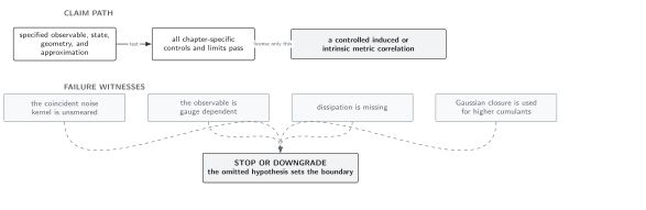
Matching $N$ fixes only second moments; tail probabilities and higher metric statistics require the corresponding renormalized stress cumulants and a controlled response expansion. The map is schematic and not to scale.

Exercises

Show that Source B above has unit variance and third cumulant $1/\sqrt2$.

Solution

Its mean is $\sqrt2/3-2/(3\sqrt2)=0$. Its second moment is $2/3+(2/3)(1/2)=1$. Since it is centered, the third cumulant is the third moment: $2\sqrt2/3-(2/3)(1/(2\sqrt2))=1/\sqrt2$.

References

• Bates, J. D. “Non-Gaussian Stochastic Gravity.” arXiv:1305.3755 [gr-qc] (2013). Stable record. Open PDF