

Cosmological Bootstrap: Loops, Initial States, Validity, and Handoffs
Tree-level Bunch–Davies reconstruction is a controlled starting point, not a universal completion. Loops add multiparticle cuts, logarithms, counterterms, and possible secular enhancement; an excited or mixed initial state adds signed-energy singularities and boundary interference; and observation adds transfer functions and nonlinear projection. Each extension preserves some structural statements and changes others.
Required background. The object dictionary, cosmological cuts, locality and field-redefinition equivalence, and reconstruction define the tree-level claims. Cosmological loops, renormalization, and secular growth and initial density matrices and boundary EFT supply the extensions.
Helpful background. Quasi-de Sitter validity sets long-time limits, and celestial and cosmological handoffs separates boundary data from later interpretation.
One-loop changes to a reconstructed tree object
Section titled “One-loop changes to a reconstructed tree object”Start from a tree-level exchange class
At one loop, a renormalized coefficient has the schematic form
The logarithm represents a branch cut rather than a tree pole. Its discontinuity,
for the declared orientation, is fixed by products of lower-order data through the loop cutting rule. The local coefficients are not fixed by that discontinuity; they absorb ultraviolet divergences and supply finite matching data. Renormalization requires
through the working order. Failure of this check exposes a missing counterterm or running coupling.
Unitarity-based cuts persist order by order for a local Hermitian theory in the Bunch–Davies state on the stated FLRW class; they do not make the full finite loop coefficient unique. Melville and Pajer’s all-loop cutting construction is the primary controlled result (Melville and Pajer 2021, revised 2026, abstract and §§ 4–5).
Late-time logarithms such as are perturbative only while their products with couplings remain small. Weinberg establishes bounds on late-time behavior under restrictions on the interactions (Weinberg 2005, §§ II–IV); outside that class, or when the logarithm becomes large, resummation or a different long-distance description is required.
Bogoliubov and finite-time initial states
Section titled “Bogoliubov and finite-time initial states”A Gaussian Bogoliubov mode is
Every external leg now contains both frequency signs. A contact integral generates phases
and hence singularities at signed energy sums , including folded configurations. Their residues carry products of and . These are state-dependent analytic data, not new flat-space particles.
Ghosh, Pajer, and Ullah derive cutting rules and a map from Bunch–Davies to Bogoliubov coefficients for IR-finite examples with interactions adiabatically switched on in the infinite past (Ghosh, Pajer, and Ullah 2025, abstract and §§ 2–4). This is a controlled extension. It does not cover every finite-time density matrix: such a state has explicit initial-boundary kernels and may break scale invariance, so its cuts must include boundary vertices and interference terms.
Backreaction and ultraviolet admissibility also constrain . The excitation energy must remain below the background budget, the short-distance state must satisfy the required adiabatic or Hadamard behavior, and boundary-EFT coefficients must remain within their cutoff expansion.
Application: test the tree reconstruction twice
Section titled “Application: test the tree reconstruction twice”Take the reconstructed and perform two deformations.
One loop. Compute the cut coefficient from tree data and independently from a direct in-in or wavefunction loop integral. Verify its branch discontinuity, regulator independence, and cancellation after local counterterms. Retain the finite as matching data.
Excited state. Replace every mode by , compute one contact and one exchange diagram, and list all signed-energy singularities with their – weights. Verify the state-specific cut against an explicit ket–bra calculation and recover the Bunch–Davies result as .
The comparison distinguishes what survives:
- Ward identities survive only with the state and slow-roll breaking sources included;
- locality still constrains allowed singularities, but the allowed state boundary action enlarges the contact space;
- perturbative unitarity survives, while the compact cut formula changes;
- the standard total-energy flat-amplitude residue remains in the Bunch–Davies component, but extra signed-energy singularities are state data;
- reconstruction remains modulo new loop counterterms and boundary operators.
Evidence classes and open boundary
Section titled “Evidence classes and open boundary”As of August 2026:
- the Gaussian coefficient–correlator inversion is an exact functional identity within its stated state;
- standard-state tree factorization and perturbative cutting rules are analytic results under their locality, branch, and FLRW hypotheses;
- Bogoliubov cutting has been demonstrated analytically in controlled IR-finite classes, not for arbitrary density matrices;
- loop cuts and renormalization are controlled order by order, while large secular effects require model-dependent resummation;
- a nonperturbative reconstruction theorem for general cosmological QFT, a universal cosmological positivity theorem, and a state-independent map to observables remain unavailable.
The final item is a boundary on the claim, not evidence against the successful controlled classes.
Second-formalism adversarial test
Section titled “Second-formalism adversarial test”For every proposed universal property, require:
- a wavefunction calculation and a closed-time-path in-in calculation;
- the Bunch–Davies limit and one admissible excited or mixed state;
- dimensional or cutoff regularization and a second regulator or renormalization check;
- the strongest known contrary fixture—an allowed contact, massless exchange, extra signed-energy singularity, or secular logarithm.
Downgrade any statement that survives only one formalism or standard-state tree level. In particular, neither a folded singularity nor a loop logarithm should be removed merely because it violates a tree rational ansatz.
The structure map shows the controlled extensions around the tree core. Inspect how loops and initial boundaries add cuts and contacts before observational projection.

Loops, initial states, infrared evolution, and observational handoffs around the cosmological-bootstrap tree core. The diagram is schematic and not to scale; each extension enlarges the analytic data and validity conditions.
The failure map prevents a mature tree identity from being promoted beyond its hypotheses. Inspect the stops for large secular logs, non-Hadamard excitations, omitted boundary cuts, and projection uncertainty.
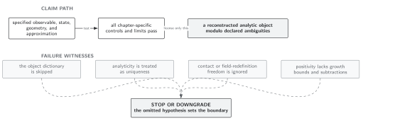
Failure conditions beyond standard-state tree level. The diagram is schematic and not to scale; controlled tree and perturbative results remain valid inside their domains without implying universal reconstruction.
These status boundaries refine the chapter’s domain and failure conditions.
Exercise
Section titled “Exercise”Compute the discontinuity of across using the boundary values .
Solution
With
the two boundary values give and , hence
for this orientation. Reversing the definition of the discontinuity reverses the sign, so the convention must accompany every cutting formula.
References
Section titled “References”- Ghosh, D., E. Pajer, and F. Ullah. “Cosmological Cutting Rules for Bogoliubov Initial States.” SciPost Physics 18 (2025): 005. DOI. Open PDF.
- Melville, S., and E. Pajer. “Cosmological Cutting Rules.” Journal of High Energy Physics 2021, no. 05 (2021): 249; arXiv revision v2 (2026), sign corrections with results unchanged. DOI. Open PDF.
- Weinberg, S. “Quantum Contributions to Cosmological Correlations.” Physical Review D 72 (2005): 043514. DOI. Open PDF.
Original QFT.org content:CC BY 4.0, unless an item supplies different terms. Third-party material retains its own terms.