Null-Projected and Smeared Stress Observables

The renormalized stress tensor is an operator-valued distribution. Its null projection becomes an operational observable only after the null direction, affine normalization, state domain, and smooth spacetime or otherwise microlocally admissible smearing are fixed. A finite one-point expectation does not make an unsmeared stress product or variance meaningful.

Required background. Renormalized Stress Tensor: Axioms and Curvature Ambiguities supplies the local tensor; Products, Scaling Degree, and Distribution Extensions supplies the product and pullback criteria.

Helpful background. Quantum Energy Inequalities supplies later bounds; Wavepackets, Modes, and Frames supplies operational localization.

Sampling a null projection

Let $\gamma(\lambda)$ be an affinely parametrized null geodesic with

$$k^\mu=\frac{\mathrm dx^\mu}{\mathrm d\lambda}, \qquad k^\nu\nabla_\nu k^\mu=0, \qquad k^\mu k_\mu=0.$$

The formal projection is $T_{kk}=T_{\mu\nu}k^\mu k^\nu$. The safe general observable is the spacetime smear

$$T[F] = \int_M\mathrm d^4x\,\sqrt{-g}\, F^{\mu\nu}(x)T_{\mu\nu}(x),$$

where $F^{\mu\nu}\in C_0^\infty$ is a symmetric test tensor concentrated in a narrow tube around $\gamma$ and aligned with a smooth extension of $k^\mu k^\nu$. Its longitudinal width, transverse width, and normalization are part of the observable.

The tempting line expression

$$\int\mathrm d\lambda\, f(\lambda)T_{\mu\nu}(\gamma(\lambda))k^\mu k^\nu$$

exists only if the pullback of the distribution to the null curve satisfies the wavefront-set criterion. For generic four-dimensional stress correlations this restriction is not automatically defined. Transverse or full spacetime smearing is therefore not optional when moments or products are required. The absence of a state-independent null-worldline quantum inequality in four-dimensional Minkowski space is a related warning, not a statement that every smeared null observable is ill-defined Fewster and Roman 2003, §§II–III, pp. 3–8.

For the fluctuation, define

$$t_{\mu\nu}(x) = T_{\mu\nu}(x)-\langle T_{\mu\nu}(x)\rangle_\omega$$

and

$$\operatorname{Var}_\omega T[F] = \frac12\int\mathrm dV_x\,\mathrm dV_y\, F^{\mu\nu}(x)F^{\rho\sigma}(y) \left\langle \{t_{\mu\nu}(x),t_{\rho\sigma}(y)\} \right\rangle_\omega.$$

This is a distributional pairing. It is nonnegative for real $F$ because it is the variance of a Hermitian smeared operator. The finite c-number curvature ambiguity in $T_{\mu\nu}$ shifts the mean but cancels from $t_{\mu\nu}$; it does not cure a forbidden coincidence limit.

First application: compact null-tube smearing

Choose local null-tube coordinates $(\lambda,v,y^A)$ around a geodesic segment and smooth compact functions

$$f_\tau(\lambda)=\frac1{\tau}f\!\left(\frac{\lambda}{\tau}\right), \qquad q_\sigma(v,y)=\frac1{\sigma^3} q\!\left(\frac v\sigma,\frac{y^1}\sigma,\frac{y^2}\sigma\right),$$

normalized in the chosen coordinate-volume approximation. Multiply by a smooth cutoff before the chart boundary and form

$$F_{\tau,\sigma}^{\mu\nu} = \mathcal N_{\tau,\sigma}\, f_\tau q_\sigma\,k^\mu k^\nu.$$

The normalization $\mathcal N_{\tau,\sigma}$ is fixed geometrically using the invariant volume form, not inferred from coordinate integrals. For a Hadamard scalar state, evaluate the one-point mean using the renormalized stress and the variance by letting the connected symmetrized stress bi-distribution act on $F_{\tau,\sigma}\otimes F_{\tau,\sigma}$.

Vary $\tau$ at fixed transverse resolution $\sigma$, then vary $\sigma$ separately. Shrinking either width probes new ultraviolet information; no pointwise limit is promised. Useful checks are compact support, reality, positivity of the variance, conservation under changes $F^{\mu\nu}\mapsto F^{\mu\nu}+\nabla^{(\mu}V^{\nu)}$ when boundary terms vanish, and stability under two tube charts describing the same tensor $F$.

Affine rescaling

Under

$$\lambda'=a\lambda,\qquad k'^\mu=\frac1a k^\mu, \qquad a>0,$$

the bare quantity $T_{kk}$ scales as $a^{-2}$. A formal line smear remains the same geometric functional only if

$$f'(\lambda')=a\,f(\lambda'/a),$$

because $\mathrm d\lambda'=a\,\mathrm d\lambda$. A separately normalized profile with $\int f\,\mathrm d\lambda=1$ transforms differently and hence defines a different weighted observable unless an additional physical normalization fixes $a$.

In a null tube, the clean procedure is to transform the complete test tensor $F^{\mu\nu}$ as a geometric object. Quoted “null energy magnitudes” that omit the affine normalization or sampling tensor are not comparable.

Adversarial coincidence and rescaling tests

First set $x=y=\gamma(\lambda)$ in the stress two-point function and only afterward try to integrate. The product contains ultraviolet singularities unsupported by the one-point subtraction, so the variance is undefined without extension or smearing.

Second rescale $k^\mu$ while leaving the displayed sampling function unchanged. The quoted mean changes by $a^{-2}$ and the variance by $a^{-4}$, even though the underlying null direction did not. The strongest surviving statement is a result for the original parametrized tangent and test tensor, not an invariant property of the unparametrized null curve.

Smearing and failure maps

The structure map places the sampling tensor before evaluation of moments and before any handoff to an energy inequality or stochastic source.

Null direction, affine scale, support, and resolution jointly define the observable; the map is schematic and not to scale.

The failure map distinguishes a finite one-point projection from an undefined product or inadmissible null pullback.

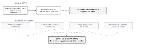
One-point renormalization, fluctuation smearing, and inequality hypotheses are separate requirements; the map is schematic and not to scale.

Use Domain and failure conditions. Record the state, null segment, affine tangent, full test tensor, longitudinal and transverse widths, support, pullback criterion if used, finite mean prescription, connected subtraction, and scaling under every normalization change.

Stress Bi-Tensors and Noise-Kernel Input constructs the separated-point covariance. Chapter 12 owns ANEC, QNEC, focusing, and QEI claims and must import the complete sampling data rather than only a number.

References

• Christopher J. Fewster and Thomas A. Roman, “Null Energy Conditions in Quantum Field Theory,” Physical Review D 67 (2003), 044003, DOI, arXiv:gr-qc/0209036.