

Adiabatic States, WKB Order, and Regularity
Adiabatic states use a high-frequency WKB expansion to choose mode data on a time-dependent background. Their order measures ultraviolet approximation or Sobolev regularity, not small particle number and not a renormalization prescription. Finite order can be adequate for a declared observable or local comparison, while the full Hadamard condition requires control to all Sobolev orders.
Required background. Covariant Scalar Fields and Curvature Coupling supplies the mode equation and the signed coupling . Vacuum Ambiguity, Time Flow, and Observer Dependence explains why an instantaneous frequency is extra structure. WKB, Eikonal Expansions, and Turning Points supplies the asymptotic method.
Helpful background. Bogoliubov Transformations and Unitary Implementability interprets changes of mode data. Asymptotic Scales, Remainders, and Uniformity clarifies why truncation order needs a regime.
WKB data in an expanding spacetime
Section titled “WKB data in an expanding spacetime”For a spatially homogeneous metric, rescale the scalar mode so that it obeys
where contains , the mass term, curvature coupling, and terms from the scale factor. The Wronskian normalization is chosen to reproduce the canonical commutator. The WKB ansatz
solves the mode equation if satisfies
Starting with , one iterates this relation and truncates according to the chosen derivative-counting convention. Initial data from define exact modes after they are evolved by the exact equation; the truncated WKB expression itself is only an asymptotic approximation.
The construction requires on the initialization surface and uniform high- control. Turning points, tachyonic bands, and zero modes need separate treatment. The site’s signed curvature coupling has conformal value in four dimensions; sources using instead quote .
What “order” controls
Section titled “What “order” controls”Iteration count, derivative order, and microlocal adiabatic order are not universally normalized, so a calculation must state its definition. A convention-independent formulation uses Sobolev wavefront sets: a quasifree state is adiabatic of order when
If is Hadamard, then
These are the precise regularity statements of Junker and Schrohe Junker and Schrohe 2002, Definition 3.2 and Lemma 3.3. Every Hadamard state is adiabatic of every finite order, but a state of one fixed finite order need not be Hadamard. Observable-dependent differentiability thresholds must be derived from Sobolev embedding rather than guessed from the label.
First application: second and fourth order
Section titled “First application: second and fourth order”On a smooth FLRW background, compute and using one stated derivative-counting convention. Let the exact evolved mode be expanded in a normalized WKB reference pair as
Then the coefficient is
Both mode families must use the same Wronskian convention. Fourth-order data cancel more terms in the large- asymptotic mismatch than second-order data. The evidence to report is the fitted high- falloff of , stability as the fitting window moves, and failures near turning points—not merely a state label.
This comparison establishes improved ultraviolet agreement. It does not prove that either finite-order state is a unique vacuum, and it does not license subtracting its entire two-point function from an observable.
State construction is not adiabatic subtraction
Section titled “State construction is not adiabatic subtraction”Adiabatic states specify initial covariance data. Adiabatic subtraction is a prescription that removes a finite set of local high-momentum terms from a composite observable. The original stress-tensor construction makes that observable-specific role explicit Parker and Fulling 1974, §§ III–IV, pp. 347–353. The order needed for a subtraction is determined by the observable and dimension; it is not inherited automatically from the order used to name a state.
The adversarial test is to take “fourth-order adiabatic state” as permission to subtract all fourth-order mode terms from any observable. That inference fails unless one separately proves the subtraction’s locality, covariance, conservation properties, and equivalence to the accepted renormalization freedom. The strongest surviving claim is finite-order ultraviolet matching of the state data.
Domain and failure conditions
Section titled “Domain and failure conditions”Adiabatic WKB data provide a controlled route from mode data toward the ultraviolet box of the construction map. A fixed finite order licenses only the associated high-frequency or Sobolev statement; it does not skip the positivity, exact evolution, or all-orders Hadamard checks.

Adiabatic order controls an ultraviolet approximation after exact mode normalization and evolution; state selection and subtraction remain separate. Schematic; not to scale.
The insufficient-regularity branch in the failure map is the decisive one. If the fitted high- remainder does not have the decay required for the claimed observable, the result must be downgraded to the lower verified order; calling the state “adiabatic” cannot supply the missing derivatives.
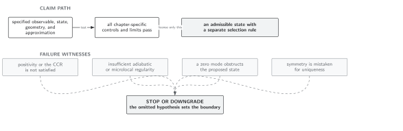
The order convention, momentum regime, and remainder estimate set the claim’s boundary; finite order is not full Hadamard control. Schematic; not to scale.
For comparison with the other state classes, see Domain and failure conditions.
Handoffs
Section titled “Handoffs”States of Low Energy and Smeared-Energy Selection uses adiabatic modes as comparison data while adding an operational sampling function. Renormalization belongs to Renormalized Stress Tensor: Axioms and Curvature Ambiguities. The relation between Sobolev order and the full Hadamard class continues in Hadamard States and Wavefront Characterization.
References
Section titled “References”- Junker, Wolfgang, and Elmar Schrohe. “Adiabatic Vacuum States on General Spacetime Manifolds: Definition, Construction, and Physical Properties.” Annales Henri Poincaré 3 (2002): 1113–1181. DOI. Open PDF.
- Parker, Leonard, and Stephen A. Fulling. “Adiabatic Regularization of the Energy-Momentum Tensor of a Quantized Field in Homogeneous Spaces.” Physical Review D 9 (1974): 341–354. DOI.
Original QFT.org content:CC BY 4.0, unless an item supplies different terms. Third-party material retains its own terms.