Differential-Form Fields and Reducible Gauge Systems

A differential-form gauge field carries local waves, a hierarchy of gauge redundancies, and global information that no local gauge condition can remove. For a $p$-form potential, the field strength is $F=\mathrm dA$, but when $p>1$ the gauge parameter itself has a gauge symmetry. Cohomology then separates propagating modes from harmonic zero modes and flux sectors, while a boundary can turn some would-be gauge transformations into charged transformations.

Required background. Curved Spacetimes, Cauchy Surfaces, and Global Hyperbolicity supplies the causal domain; Gauge Fields, Gauge Fixing, and Ghosts on Curved Backgrounds supplies the gauge-field prototype; Differential Forms, Integration, and Stokes’ Theorem supplies exterior calculus.

Helpful background. Presymplectic Systems and the Covariant Phase-Space Ambiguity Map explains gauge degeneracy; The BV Formalism and Gauge Fixing organizes reducible symmetries; Metrics, Volume Forms, Hodge Stars, and Laplace-Type Operators supplies the Hodge decomposition.

Form fields and their gauge tower

Let $A\in\Omega^p(M)$ be an Abelian $p$-form potential and

$$F=\mathrm dA\in\Omega^{p+1}(M).$$

The free action is

$$S[A] = -\frac12\int_M F\wedge *F,$$

with an overall sign fixed so that the propagating modes have positive energy in the global $(+---)$ convention. Its bulk Euler–Lagrange equation and Bianchi identity are

$$\delta F=0, \qquad \mathrm dF=0,$$

where $\delta$ is the metric codifferential. The potential description is invariant under

$$A\longmapsto A+\mathrm d\Lambda_{p-1}.$$

For $p=1$ the gauge parameter is a scalar. For $p\ge2$, however,

$$\Lambda_{p-1}\longmapsto \Lambda_{p-1}+\mathrm d\Lambda_{p-2}$$

does not change $A$. The $(p-2)$-form parameter is itself reducible, and the sequence continues down to degree zero. In BRST or BV quantization this produces ghosts, ghosts-for-ghosts, and alternating statistics along the tower. A single Faddeev–Popov scalar therefore cannot represent a reducible $p$-form system.

The Lorenz condition $\delta A=0$ converts the potential equation into a de Rham wave equation,

$$( \mathrm d\delta+\delta\mathrm d )A=0,$$

whose principal part is normally hyperbolic. This is a local propagation statement. Harmonic forms, non-exact fluxes, residual gauge transformations, and boundary modes remain to be treated globally.

Propagating modes, harmonic modes, and flux

On a compact Riemannian Cauchy surface $\Sigma$ without boundary, Hodge theory gives

$$\Omega^p(\Sigma) = \operatorname{im}\mathrm d \oplus \operatorname{im}\delta_\Sigma \oplus \mathcal H^p(\Sigma).$$

The exact part is locally gauge, the coexact part contains transverse propagating data, and the harmonic subspace $\mathcal H^p(\Sigma)$ has dimension $b_p(\Sigma)$. Its coefficients are finite-dimensional zero modes. A nonzero cohomology class of $F$ is a flux sector; if $[F]\ne0$, no single globally defined potential $A$ represents that sector.

This decomposition depends on the global slice and on boundary conditions. It is not a pointwise polarization decomposition. In particular, two spacetimes can be locally isometric and have identical curvature invariants while possessing different Betti numbers and different global observable algebras.

For the gauge-fixed functional integral, zero modes must be removed from determinants and integrated or summed with their correct finite-dimensional measure. The formal expression

$$\det{}'(\Delta_k)$$

uses a prime precisely because the harmonic kernel has been separated. Ignoring it can produce a vanishing determinant, an infinite gauge volume, or the wrong topological dependence.

First application: a free two-form on a compact slice

Consider a two-form $B$ in four spacetime dimensions,

$$H=\mathrm dB, \qquad B\longmapsto B+\mathrm d\Lambda_1, \qquad \Lambda_1\longmapsto\Lambda_1+\mathrm d\lambda.$$

On an ultrastatic spacetime $\mathbb R\times\Sigma$, decompose the spatial two-form as

$$B_\Sigma = \mathrm d\alpha +\delta_\Sigma\beta +\sum_{I=1}^{b_2}q^I(t)\,\omega_I,$$

where $\omega_I$ are harmonic two-forms. The exact term is gauge; the coexact term carries the local wave modes. The coefficients $q^I$ are global degrees of freedom whose velocities contribute electric-type harmonic flux. A magnetic three-form flux belongs to $H^3(\Sigma)$ and can obstruct a global potential.

Take $\Sigma=T^3$. Then $b_1=3$, $b_2=3$, and $b_3=1$. The two-form therefore has harmonic zero modes and a possible three-form flux sector in addition to its local propagating mode. Its one-form gauge parameter also has harmonic zero modes, and the scalar reducibility parameter removes only its exact redundancy. Gauge fixing must divide by this finite-dimensional stabilizer separately from the nonzero modes.

Locally, a massless two-form in four dimensions is dual to a scalar:

$$H=*\,\mathrm d\varphi.$$

The duality is exact only after matching zero modes, flux quantization, periodicities, and boundary conditions. Equality of the local wave equations is not sufficient to identify the global theories.

Boundary observables and the adversarial topology test

Varying the action produces the boundary contribution

$$\delta S\big|_{\partial M} = -\int_{\partial M}\delta A\wedge *F.$$

A well-posed theory must therefore fix compatible electric-type data, magnetic-type data, or a mixed condition, possibly with added boundary degrees of freedom. A gauge parameter that is nonzero at the boundary can change a boundary charge. Whether it is quotiented out is part of the theory, not a consequence of the bulk equation.

Now compare $\mathbb R\times\mathbb R^3$ with a large flat region inside $\mathbb R\times T^3$. The local metric and all local curvature tensors can agree, so a local mode calculation gives the same short-distance propagating sector. Yet $T^3$ has harmonic one- and two-forms and a nontrivial top form, whereas $\mathbb R^3$ has no corresponding compact-cycle fluxes. The local calculation therefore misses precisely the harmonic modes, holonomies, and superselection data. Fewster and Lang exhibit this mechanism rigorously for the Maxwell field: nontrivial de Rham cohomology can create radicals classically and central observables quantum mechanically Fewster and Lang 2015, §§3–6.

The conclusion has a sharp ceiling: local $p$-form propagation is controlled by a Green-hyperbolic gauge-fixed operator, but the full quantum theory is not determined until the cohomology, flux lattice, gauge stabilizers, and boundary conditions are specified.

Construction and failure maps

The construction diagram locates reducible gauge reduction between the form-valued wave operator and the physical algebra. For a $p$-form, that stage includes the entire gauge-for-gauge tower and the harmonic sector.

The physical $p$-form solution space combines propagating coexact modes with separately treated harmonic and flux data; the map is schematic and not to scale.

The failure map applies most directly to ignored zero modes and boundary flux. A determinant over nonzero modes can be correct while the full partition function or observable algebra is still wrong.

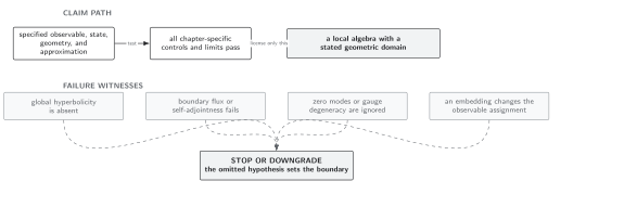
Local propagation licenses only the radiative sector until the cohomology, gauge stabilizers, flux lattice, and boundary problem have also passed; the map is schematic and not to scale.

The common comparison is in Domain and failure conditions. The page-specific decisive data are the form degree, reducibility complex, Hodge kernels, global flux class, allowed gauge group, determinant zero-mode prescription, and boundary flux.

Check your understanding

For a three-form potential $C$ with $\delta C=0$, list the reducibility tower.

Solution

The gauge transformation is $C\mapsto C+\mathrm d\Lambda_2$. It is unchanged under $\Lambda_2\mapsto\Lambda_2+\mathrm d\Lambda_1$, while the one-form parameter is unchanged under $\Lambda_1\mapsto\Lambda_1+\mathrm d\lambda$. The BRST complex therefore requires a two-form ghost, a one-form ghost-for-ghost, and a scalar ghost-for-ghost-for-ghost, with alternating Grassmann parity. Harmonic representatives at each degree are not removed by these exact transformations and require separate treatment.

The analytic construction of Green operators belongs to Green Operators, Causal Propagators, and State-Dependent Two-Point Functions. General cohomology and Hodge theory remain in Volume I; systematic reducible gauge quantization remains in Volume III; topological phases and extended observables require their own specialist treatment.

References

• Marco Benini, “Optimal Space of Linear Classical Observables for Maxwell $k$-Forms via Spacelike and Timelike Compact de Rham Cohomologies,” Journal of Mathematical Physics 55 (2014), 053502, DOI, arXiv:1401.7563.
• Christopher J. Fewster and Benjamin Lang, “Dynamical Locality of the Free Maxwell Field,” Annales Henri Poincaré 17 (2016), 401–436, DOI, arXiv:1403.7083.
• Albert Schwarz, “The Partition Function of Degenerate Quadratic Functional and Ray–Singer Invariants,” Letters in Mathematical Physics 2 (1978), 247–252, DOI.