Adiabatic Particle Number in Cosmology

Adiabatic particle number compares an exact normalized mode with a finite-order WKB basis in phase space. It becomes a controlled late-time diagnostic when a common adiabatic out region exists. During the evolution it depends on the chosen canonical variable, phase convention, and truncation order; that dependence is part of the uncertainty, not a physical production history.

Required background. FLRW mode quantization fixes the symplectic normalization; adiabatic states fixes the WKB hierarchy; particle observables fixes the operational caveat; and Stokes production treats turning points. Helpful background. Time-dependent particle creation develops exact in/out comparisons.

WKB bases are phase-space comparisons

For

$$v_k''+\Omega_k^2v_k=0, \qquad v_kv_k^{*'}-v_k'v_k^*=i,$$

introduce the normalized comparison function

$$w_k^{[r]}(\eta)= \frac{1}{\sqrt{2W_k^{[r]}(\eta)}} \exp\!\left[-i\int^\eta W_k^{[r]}(u)\,du\right].$$

Iterating

$$W_k^2=\Omega_k^2 -\frac12\frac{W_k''}{W_k} +\frac34\left(\frac{W_k'}{W_k}\right)^2$$

and retaining derivatives through order $r$ defines $W_k^{[r]}$. At a given time, match both the mode and its derivative:

$$v_k=\alpha_k^{[r]}w_k^{[r]} +\beta_k^{[r]}w_k^{[r]*}, \qquad v_k'=\alpha_k^{[r]}w_k^{[r]\prime} +\beta_k^{[r]}w_k^{[r]*\prime}.$$

The symplectic projections are

$$\alpha_k^{[r]} =-i\left(v_kw_k^{[r]*\prime}-v_k'w_k^{[r]*}\right), \qquad \beta_k^{[r]} =i\left(v_kw_k^{[r]\prime}-v_k'w_k^{[r]}\right).$$

Because a truncated $w_k^{[r]}$ is not generally an exact global solution, $\alpha_k^{[r]}(\eta)$ and $\beta_k^{[r]}(\eta)$ are instantaneous phase-space coordinates. Only in a stationary or sufficiently adiabatic asymptotic region do they settle into ordinary constant Bogoliubov coefficients. This qualification prevents a local WKB expansion from being mistaken for an exact decomposition in the solution space.

The nominal occupation is

$$n_k^{[r]}(\eta)=|\beta_k^{[r]}(\eta)|^2.$$

Successive orders estimate a remainder only while the derivative hierarchy is small. The WKB series is generally asymptotic, so increasing $r$ beyond the optimal order eventually worsens the approximation. Winitzki quantifies this limitation for cosmological particle production Winitzki 2005, §II, while Dabrowski and Dunne show how optimal truncation organizes the basis-dependent intermediate-time profile Dabrowski and Dunne 2016.

Exact FLRW pulse benchmark

Choose a massive conformally coupled scalar, $\xi=-1/6$, in the smooth spatially flat geometry

$$a^2(\eta)=a_0^2 \left[1+\varepsilon\operatorname{sech}^2(\eta/\tau)\right], \qquad \varepsilon>0.$$

The scale factor begins and ends at $a_0$ and executes a smooth expansion–contraction pulse. Define

$$x=\frac\eta\tau, \qquad q=\tau\sqrt{k^2+m^2a_0^2}, \qquad g=\varepsilon m^2a_0^2\tau^2, \qquad u_k(x)=\frac{v_k(\tau x)}{\sqrt\tau}.$$

The dimensionless mode has $x$-Wronskian $u_ku_{k,x}^*-u_{k,x}u_k^*=i$. Its exact equation is the Pöschl–Teller problem

$$\frac{d^2u_k}{dx^2} +\left[q^2+g\operatorname{sech}^2x\right]u_k=0.$$

Positive-frequency data at $x\to-\infty$ evolve into

$$u_k\longrightarrow \frac{\alpha_ke^{-iqx}+\beta_ke^{iqx}}{\sqrt{2q}} \quad (x\to+\infty).$$

Let

$$g=\lambda(\lambda+1), \qquad \lambda=\frac{\sqrt{1+4g}-1}{2}.$$

Hypergeometric connection gives the exact late occupation

$$n_{k,\mathrm{exact}}^{\rm out} =\frac{\sin^2(\pi\lambda)}{\sinh^2(\pi q)}.$$

For the associated spatial scattering problem,

$$R=\frac{\sin^2(\pi\lambda)} {\sinh^2(\pi q)+\sin^2(\pi\lambda)}, \qquad T=\frac{\sinh^2(\pi q)} {\sinh^2(\pi q)+\sin^2(\pi\lambda)}.$$

The time-dependent oscillator has the hyperbolic normalization $|\alpha|^2-|\beta|^2=1$, so its occupation is $|\beta|^2=R/T$, not the spatial reflection probability $R$. The solvable potential originates with Pöschl and Teller 1933.

This is an actual massive FLRW calculation, not an abstract oscillator with an undeclared geometric origin. The massless conformal limit gives $g=0$ and hence $\beta_k=0$, reproducing the negative control of the preceding page.

For weak amplitude $g\ll1$, with $g\ll q^2$ also ensuring a small local-frequency perturbation, first-order retarded perturbation theory gives

$$\begin{aligned} \beta_k^{(1)} &=\frac{i}{2\omega_k} \int_{-\infty}^{\infty}d\eta\, \delta V\operatorname{sech}^2(\eta/\tau)e^{-2i\omega_k\eta}\\ &=\frac{i\pi\delta V\tau^2} {\sinh(\pi\omega_k\tau)}, \end{aligned}$$

where $\omega_k=q/\tau$ and $\delta V=g/\tau^2$. The plus sign follows from the page’s conventions for $w_k$, $\beta_k$, and the out expansion. A different out-mode phase can rotate $\beta_k$, but it must be changed consistently when transitions interfere. The Born occupation is

$$n_{k,\mathrm{Born}}^{\rm out} =\frac{\pi^2g^2}{\sinh^2(\pi q)}.$$

The figure shows a frozen benchmark at $g=0.02$. It compares direct mode evolution against the exact and Born results; the machine-readable files record the numerical and canonical residuals.

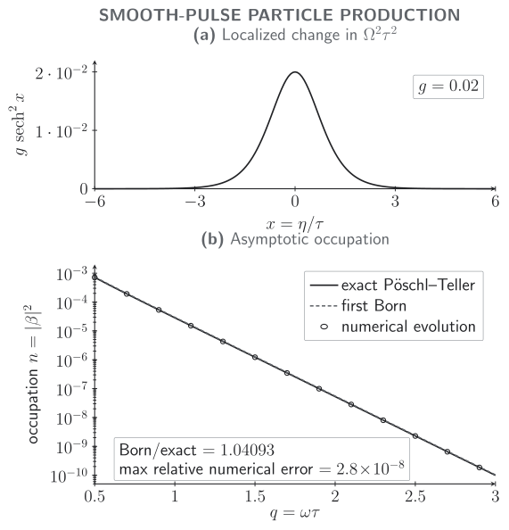
For $x=\eta/\tau$, $q=\omega\tau$, and $g=\delta V\tau^2=0.02$, numerical evolution from $x=-12$ to $12$ reproduces $n_{\rm exact}=\sin^2(\pi\lambda)/\sinh^2(\pi q)$, with $\lambda(\lambda+1)=g$. The Born curve captures the exponential adiabatic suppression and is $4.09\%$ high at this finite $g$. Every plotted point satisfies the recorded Wronskian, Bogoliubov-unitarity, domain, and tolerance checks. Quantitative; no fitted data.

Download the plotted data as CSV or inspect the machine-readable verification record.

What successive adiabatic orders establish

For this pulse, every derivative of $a$ vanishes as $x\to\pm\infty$. Consequently,

$$W_k^{[0]}=W_k^{[2]}=W_k^{[4]}=\omega_k$$

in both asymptotic regions. Zeroth-, second-, and fourth-order phase-space projections therefore give the same exact late occupation. Their agreement is not a numerical miracle: the comparison bases have become identical. At finite $x$, by contrast, the three $W_k^{[r]}$ differ and so do the corresponding $n_k^{[r]}(x)$.

Comparison	Meaning
Orders $0,2,4$ agree in the common out region	The late particle interpretation is stable under these basis refinements.
Orders disagree during the pulse	The spread estimates basis and truncation dependence; it is not an error bar on an observable production history.
Direct evolution disagrees with the exact formula	The integration domain, time step, Wronskian, or projection convention has failed.
Exact and Born curves disagree at finite $g$	This is the controlled perturbative remainder, not numerical error.

The reproducibility contract separates four uncertainties. Numerical error is tested by the differential-equation residual, Wronskian, $|\alpha|^2-|\beta|^2=1$, step refinement, and increasing the domain from $|x|=12$. Adiabatic uncertainty is the sensible-order spread in a region with small derivatives. Perturbative uncertainty is measured here against the exact Pöschl–Teller answer. Model uncertainty comes from varying $a(\eta)$, $m$, and $\xi$; it must not be hidden inside solver tolerance.

Near a turning point with $\Omega_k^2=0$, the local WKB hierarchy fails even though the exact mode remains regular. Uniform approximations or Stokes analysis must then connect controlled regions. For a spectrum, convergence must also be uniform enough under the $k$ integral: agreement of a few infrared modes does not control a high-$k$ tail that can dominate the energy.

Common pitfalls

Projecting the field amplitude without its derivative. One complex amplitude at one instant does not determine a phase-space direction. The symplectic formulas use both $v_k$ and $v_k'$ and expose normalization errors.

Interpreting order-by-order oscillations as particles appearing and disappearing. Intermediate $n_k^{[r]}$ changes when the adiabatic basis or canonical variable changes. The controlled result here is the common asymptotic coefficient.

Exercises

1. Derive the Born coefficient

Use the retarded Green function of $d^2/d\eta^2+\omega^2$ to derive the first-order coefficient for $V(\eta)=\delta V\operatorname{sech}^2(\eta/\tau)$.

Solution

With incoming mode $w=e^{-i\omega\eta}/\sqrt{2\omega}$, the first correction is

$$\delta v(\eta)= -\int_{-\infty}^{\eta}ds\, \frac{\sin[\omega(\eta-s)]}{\omega}V(s)w(s).$$

The coefficient of the late $e^{+i\omega\eta}/\sqrt{2\omega}$ term is

$$\beta^{(1)}=\frac{i}{2\omega} \int_{-\infty}^{\infty}ds\,V(s)e^{-2i\omega s}.$$

Using

$$\int_{-\infty}^{\infty}d\eta\, \operatorname{sech}^2(\eta/\tau)e^{-2i\omega\eta} =\frac{2\pi\omega\tau^2}{\sinh(\pi\omega\tau)}$$

gives $\beta^{(1)}=i\pi\delta V\tau^2/\sinh(\pi\omega\tau)$.

2. Find a failure of the weak-pulse approximation

The exact result is reflectionless when $\lambda$ is a positive integer. Compare the exact and Born predictions at $g=2$.

Solution

For $g=2$, $\lambda(\lambda+1)=2$ gives $\lambda=1$. Hence

$$n_{\rm exact}=\frac{\sin^2\pi}{\sinh^2(\pi q)}=0.$$

The Born expression instead gives $4\pi^2/\sinh^2(\pi q)$, which is nonzero. There is no contradiction: $g=2$ is far outside the weak-pulse regime. The exact cancellation is nonperturbative in the pulse strength, so this case is a deliberate negative control on extrapolating the first-order formula.

References

• Dabrowski, Robert, and Gerald V. Dunne. “Superadiabatic Particle Number in Schwinger and de Sitter Particle Production.” Physical Review D 90 (2014): 025021. DOI.
• Dabrowski, Robert, and Gerald V. Dunne. “Time Dependence of Adiabatic Particle Number.” Physical Review D 94 (2016): 065005. DOI.
• Parker, Leonard. “Quantized Fields and Particle Creation in Expanding Universes. I.” Physical Review 183 (1969): 1057–1068. DOI.
• Pöschl, G., and E. Teller. “Bemerkungen zur Quantenmechanik des anharmonischen Oszillators.” Zeitschrift für Physik 83 (1933): 143–151. DOI.
• Winitzki, Sergei. “Cosmological Particle Production and the Precision of the WKB Approximation.” Physical Review D 72 (2005): 104011. DOI. Open PDF.