Gauge-Invariant Stochastic Observables

A covariance of metric components is not yet a gravitational observable: $h_{\mu\nu}$ changes under an infinitesimal diffeomorphism. Stochastic gravity becomes predictive only after the response is projected onto a gauge-invariant or relational quantity and smeared over a finite spacetime region. This page constructs a compactly supported linearized-curvature observable and shows how its variance loses all dependence on the metric gauge.

Required background. Intrinsic and Induced Metric Fluctuations supplies the covariance decomposition, while Gauge-Invariant Response Kernels supplies constraint-compatible projection.

Helpful background. Relative Cauchy Evolution and Background Response relates metric variation to observables, and Null-Smeared Stress Observables illustrates why the smearing domain matters.

Gauge transformations and observable choices

At linear order,

$$h_{\mu\nu}\longmapsto h_{\mu\nu}+2\nabla_{(\mu}\zeta_{\nu)}.$$

A stochastic two-point function $\mathbb E[h_{\mu\nu}(x)h_{\rho'\sigma'}(y)]$ therefore changes when the gauge-fixing Green function changes. Three standard routes remove this redundancy.

1. Project scalar, vector, and tensor perturbations onto gauge-invariant combinations when the background symmetry permits it.
2. Use a tensor whose background value vanishes. Its first-order perturbation is gauge invariant because $\delta_\zeta A^{(1)}=\mathcal L_\zeta A^{(0)}=0$.
3. Define coordinates relationally using physical clock and rod fields, then perturb the quantity at fixed clock values.

For example, on a conformally flat background $C^{(0)}_{\mu\nu\rho\sigma}=0$, so the linearized Weyl tensor is gauge invariant. On a generic background it transforms by $\mathcal L_\zeta C^{(0)}$ and needs a relational completion or another invariant. This is an application of the Stewart–Walker criterion Stewart and Walker 1974, pp. 51–55, not a claim that every curvature perturbation is gauge invariant.

The structure map makes gauge reduction a stage after causal propagation inputs but before comparison with quantum correlators. Inspect the output node: it is a smeared curvature or relational observable, never a bare coordinate component.

Gauge fixing helps invert the response operator, but only the projected observable and its finite-support covariance may be exported. The map is schematic and not to scale.

First application: smeared linearized curvature

On Minkowski spacetime, where the background Riemann tensor vanishes, define

$$R^{(1)}_{\mu\nu\rho\sigma}[h] =\frac12\left( \partial_\rho\partial_\nu h_{\mu\sigma} +\partial_\sigma\partial_\mu h_{\nu\rho} -\partial_\sigma\partial_\nu h_{\mu\rho} -\partial_\rho\partial_\mu h_{\nu\sigma} \right).$$

Substituting $\delta h_{\mu\nu}=2\partial_{(\mu}\zeta_{\nu)}$ makes all third derivatives cancel pairwise. Let $F^{\mu\nu\rho\sigma}\in C_0^\infty$ have the algebraic symmetries of the Riemann tensor and support in a finite causal diamond $D$. The observable

$$\mathcal R[F] =\int_D\mathrm d^4x\, F^{\mu\nu\rho\sigma}(x) R^{(1)}_{\mu\nu\rho\sigma}[h](x)$$

is therefore invariant under compactly supported linearized diffeomorphisms.

For the induced solution $h=8\pi G\,G^{\mathrm{ret}}\xi$, integrate derivatives by parts and define the effective stress sampler

$$K_F^{\alpha\beta}(y) =\int_D\mathrm d^4x\, F^{\mu\nu\rho\sigma}(x) \mathcal R_{\mu\nu\rho\sigma}^{\phantom{\mu\nu\rho\sigma}\gamma\delta} G^{\mathrm{ret}}_{\gamma\delta}{}^{\alpha\beta}(x,y),$$

where $\mathcal R$ is the linearized Riemann differential operator. Then

$$\mathcal R^{\mathrm{ind}}[F] =8\pi G\,\xi(K_F), \qquad \operatorname{Var}\mathcal R^{\mathrm{ind}}[F] =(8\pi G)^2N(K_F,K_F).$$

$K_F(y)$ vanishes outside the causal past of $D$ for a retarded response. In a finite initial-value region it is an admissible past-compact sampler, and the variance is nonnegative. The four derivatives implicit in the two curvature insertions are applied distributionally; compact support and the renormalized contact prescription are part of the observable.

Two-gauge comparison

Compute the response in two gauges, with Green functions related schematically by

$$G^{\mathrm{ret},'}_{\mu\nu}{}^{\alpha\beta} =G^{\mathrm{ret}}_{\mu\nu}{}^{\alpha\beta} +2\partial_{(\mu}Y_{\nu)}{}^{\alpha\beta} +G^{\mathrm{constr}}_{\mu\nu}{}^{\alpha\beta}.$$

The pure-gauge term is annihilated by $\mathcal R$. The constraint term vanishes against a conserved source only after the linearized constraints and stress contact terms are included. Thus

$$K_F'=K_F, \qquad \operatorname{Var}'\mathcal R[F] =\operatorname{Var}\mathcal R[F].$$

If the two calculations disagree, the difference diagnoses a missing constraint mode, boundary term, or contact contribution—not stochastic gauge dependence of the physical curvature. Cosmological implementations use the same logic for Bardeen variables and reproduce the corresponding quantum metric correlations in the controlled linear model Roura and Verdaguer 2008, §§II–IV.

For a generic curved background and a scalar clock $X=X_0+\delta X$, a scalar observable $A=A_0+\delta A$ has the first-order relational completion

$$\delta A_{X} =\delta A-\frac{\delta X}{K^\mu\nabla_\mu X_0} K^\nu\nabla_\nu A_0,$$

along a declared background flow $K$. The two terms transform oppositely for gauge displacements along that flow, or when the relevant background gradients are aligned with it. One scalar clock does not cancel an arbitrary spacetime diffeomorphism: a generic relational construction needs enough independent clock-and-rod fields. The displayed construction is also local to the region where the clock gradient is nonzero; nonperturbative relational observables are not supplied by the linear stochastic model.

Domain and failure conditions

The chapter comparison table licenses variances of declared gauge-invariant observables with finite spacetime smearing, conserved noise, solved constraints, a retarded domain, and fixed boundary conditions. A coordinate-space power spectrum of $h_{\mu\nu}$ is not automatically such an observable. Detector readout adds an operational coupling and belongs to the curved-channels treatment.

The failure map’s gauge-dependent branch is tested directly by the two-gauge calculation above.

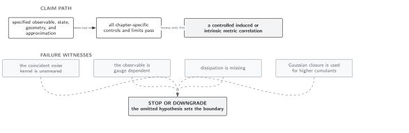
Gauge agreement of the curvature variance is a reproducible acceptance test; disagreement forces repair of constraints, boundary terms, or renormalized contacts. The map is schematic and not to scale.

References

• Roura, A., and E. Verdaguer. “Cosmological Perturbations from Stochastic Gravity.” Physical Review D 78, 064010 (2008). doi:10.1103/PhysRevD.78.064010. Open PDF
• Stewart, J. M., and M. Walker. “Perturbations of Spacetimes in General Relativity.” Proceedings of the Royal Society A 341, 49–74 (1974). doi:10.1098/rspa.1974.0072