Entanglement Harvesting in Curved Spacetime

Entanglement harvesting transfers field correlations into initially uncorrelated localized probes. In curved spacetime the result depends jointly on geometry, field state, trajectories, separation, switching, smearing, detector gaps, and perturbative control. Curvature has no universal sign: it can change both the nonlocal coherence that supports entanglement and the local excitation that competes with it.

Required background. Curved-Spacetime Channel Deployment Contract fixes the operational data. Switching, Smearing, Finite-Time Response, and Transients controls local probe response. Vacuum Entanglement Harvesting supplies the flat-space perturbative construction.

Helpful background. Correlation Extraction versus Causal Exchange distinguishes harvesting from interaction-mediated generation. Hadamard Admissibility and the Two-Point Wavefront Criterion controls the two-point singularity.

Two-probe perturbation theory

Let two initially uncorrelated two-level probes begin in $|g_Ag_B\rangle$ and couple to a scalar field through

$$H_I(\tau)=\sum_{\nu=A,B} \lambda_\nu\chi_\nu(\tau_\nu) \left( \sigma_\nu^+e^{i\Omega_\nu\tau_\nu} +\sigma_\nu^-e^{-i\Omega_\nu\tau_\nu} \right) \Phi(F_\nu,\tau_\nu).$$

Smooth compact switching and smearing make every integral an honest pairing with the two-point distribution. To second order, the reduced detector state has the X-state form

$$\rho_{AB}= \begin{pmatrix} 1-\mathcal L_{AA}-\mathcal L_{BB}&0&0&\mathcal M^*\\ 0&\mathcal L_{BB}&\mathcal L_{AB}^*&0\\ 0&\mathcal L_{AB}&\mathcal L_{AA}&0\\ \mathcal M&0&0&0 \end{pmatrix} +O(\lambda^4).$$

The local excitation and single-excitation coherence are

$$\mathcal L_{\mu\nu} =\lambda_\mu\lambda_\nu \int d\tau\,d\tau'\, \chi_\mu(\tau)\chi_\nu(\tau') e^{-i\Omega_\mu\tau+i\Omega_\nu\tau'} \omega_2(F_\mu,\tau;F_\nu,\tau'),$$

while $\mathcal M$ contains the time-ordered pair of excitation terms. Its explicit step functions depend on the chosen common time used in the Dyson ordering, but the final covariant result does not. For identical detectors, the leading negativity is

$$\mathcal N^{(2)}=\max\{0,|\mathcal M|-\mathcal L_{AA}\}.$$

For unequal local noise,

$$\mathcal N^{(2)} =\max\!\left\{0, \frac{ \sqrt{(\mathcal L_{AA}-\mathcal L_{BB})^2+4|\mathcal M|^2} -\mathcal L_{AA}-\mathcal L_{BB}}{2} \right\}.$$

These formulas display the competition directly. Geometry and state can increase $|\mathcal M|$, increase local noise, or do both. The standard perturbative framework and its dependence on detector profiles are analyzed in Pozas-Kerstjens and Martín-Martínez 2015, §§ II–III.

Ultrastatic curved application

Take

$$ds^2=dt^2-h_{ij}(\mathbf x)dx^idx^j$$

with compact or suitably controlled spatial section and positive spatial operator

$$A=-\Delta_h+m^2+\xi R, \qquad A\psi_j=\omega_j^2\psi_j.$$

In the ultrastatic ground state,

$$\omega_2(t,\mathbf x;t',\mathbf x') =\sum_j\frac{ e^{-i\omega_j(t-t'-i0)}}{2\omega_j} \psi_j(\mathbf x)\overline{\psi_j(\mathbf x')}.$$

Smear each detector with $F_A,F_B$ and define $F_{\nu j}=\int d\mathrm{vol}_h F_\nu\psi_j$. For identical stationary detectors with switching $\chi$, the local term becomes

$$\mathcal L_{AA} =\lambda^2\sum_j\frac{|F_{Aj}|^2}{2\omega_j} \left| \widehat\chi(\Omega+\omega_j) \right|^2,$$

and the nonlocal terms contain $F_{Aj}\overline{F_{Bj}}$ with the corresponding ordered switching transform. This mode sum is a reproducible calculation once the spatial spectrum, state, detector locations, widths, gap, and switching are fixed.

Choose the compact supports to be spacelike separated. Then $E(F_A,F_B)=0$ throughout the interaction and direct causal exchange is absent. Compute $\mathcal N^{(2)}$ and compare it with a flat fixture matched by:

• equal detector proper gaps and proper switching durations;
• equal smearing profiles in local orthonormal frames;
• equal geodesic separation relative to the detector width;
• the analogous ground or Hadamard state;
• equal perturbative coupling norm.

The difference then records the combined effect of the curved spatial spectrum and state correlations for this fixture. It is not a sign-definite functional of scalar curvature. Black-hole detector studies likewise find location- and state-dependent behavior rather than a universal degradation law Henderson et al. 2018, §§ 3–5.

Perturbative and causal checks

Several checks are compulsory:

1. The $O(\lambda^2)$ excitation probabilities must remain much smaller than one, and omitted $O(\lambda^4)$ terms must not be comparable to the small positive negativity.
2. The field state must be Hadamard, or the smearing and detector model must explicitly justify any weaker singularity class.
3. Spacelike separation must hold for the full worldtubes, not only their central events.
4. The flat comparison must match proper detector data; holding coordinate width fixed can introduce a spurious curvature trend.
5. A positive partial-transpose test establishes detector entanglement only for the calculated reduced state; it does not measure all field entanglement or Bell nonlocality.

Refuting universal degradation

The adversarial statement “curvature degrades harvesting” is tested by varying one declared input at a time. Change the state within the Hadamard class, move the detectors while preserving proper separation, change their trajectories, or compensate the local gaps for redshift. Enhancement, suppression, and nonmonotonicity are all possible because $\mathcal M$ and $\mathcal L_{\nu\nu}$ sample different combinations of the two-point function. The strongest surviving statement is conditional: for the specified geometry, state, profiles, and comparison rule, the computed negativity is larger or smaller than the matched fixture.

Domain, limits, and maps

See Domain and failure conditions. The calculation above is a leading-order detector-model result. It does not establish a nonperturbative distillation rate, an experimentally available instrument, or a curvature monotonicity theorem. Timelike or tail-connected supports require the exchange decomposition on the next page.

The structure map locates harvesting after state-controlled propagation and before the task metric. Inspect the state covariance contribution: it is the resource sampled by spacelike probes.

Harvesting compares the nonlocal coherence built from the two-point function with local detector excitation under fully specified geometry and profiles. Schematic; not to scale.

The failure map warns that a causal contribution changes the interpretation. For genuinely spacelike supports the commutator test vanishes; otherwise the result must be decomposed.

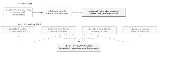
Negativity alone does not identify its origin; commutator support and matched local controls determine whether “harvested” is licensed. Schematic; not to scale.

Handoffs

Correlation Extraction versus Causal Exchange on Curved Backgrounds treats nonzero commutator contributions. Horizon-Restricted Local Operations and Distillability asks which extracted resource is operationally accessible. Abstract harvesting theory remains with Vacuum Entanglement Harvesting.

References

• Henderson, Laura J., Robie A. Hennigar, Robert B. Mann, Alexander R. H. Smith, and Jialin Zhang. “Harvesting Entanglement from the Black Hole Vacuum.” Classical and Quantum Gravity 35 (2018): 21LT02. DOI. Open PDF.
• Pozas-Kerstjens, Alejandro, and Eduardo Martín-Martínez. “Harvesting Correlations from the Quantum Vacuum.” Physical Review D 92 (2015): 064042. DOI. Open PDF.
• Reznik, Benni. “Entanglement from the Vacuum.” Foundations of Physics 33 (2003): 167–176. DOI. Open PDF.