Black-Hole Evaporation and Mean Backreaction

Hawking flux on a fixed black-hole background supplies a source candidate, not an evaporating spacetime. Mean backreaction requires a state and renormalized stress tensor on the evolving geometry, all stress components needed by the constraints, and a causal update of that same geometry. In the large-mass, slowly evolving regime, a greybody-resolved Unruh-state luminosity can drive a controlled quasi-stationary mass law. That approximation must stop before it is used to infer an endpoint.

Required background. The semiclassical Einstein equation defines the mean source; evaporating backgrounds and adiabatic backreaction supplies the slowly evolving horizon approximation; and quantum-state evolution on backreacted backgrounds makes the state update part of the coupled problem.

Helpful background. Hawking stress flux in two-dimensional reductions supplies controlled lower-dimensional examples, while black-hole states, greybody factors, and flux separates state, scattering, and asymptotic observables.

From a fixed-background luminosity to a mean mass law

For a large, neutral, nonrotating hole with slowly varying mass $M(u)$, define the instantaneous surface gravity and temperature

$$\kappa(u)=\frac{1}{4M(u)}, \qquad T_{\mathrm H}(u)=\frac{\kappa(u)}{2\pi}.$$

On a stationary Schwarzschild background, the Unruh-state luminosity at future null infinity is

$$L_\infty(M) =\sum_{s,\ell,m} \int_0^\infty\frac{d\omega}{2\pi}\, \frac{\omega\,\Gamma_{s\ell m}(\omega;M)} {\exp[\omega/T_{\mathrm H}(M)]-(-1)^{2s}},$$

where $\Gamma_{s\ell m}$ is the transmission probability through the exterior potential. Page’s numerical greybody calculation established the species-dependent emission rates on a fixed Schwarzschild geometry (Page 1976, Tables I–VI). Replacing $\Gamma$ by one changes the flux even when the near-horizon occupation factor is thermal.

Energy balance motivates

$$\frac{dM}{du}=-L_\infty[M(u)].$$

For massless species $L_\infty\simeq\alpha/M^2$, with $\alpha$ determined by the field content and greybody factors, so

$$M^3(u)\simeq M_0^3-3\alpha(u-u_0).$$

This ordinary differential equation is the leading quasi-static reduction. It does not determine the full renormalized tensor in the exterior or interior. Local conservation relates the positive outward flux at infinity to an ingoing negative Killing-energy flux near the future horizon, but the interpolation also contains vacuum-polarization components. The Unruh state is regular on the future horizon and radiating at infinity; the Hartle–Hawking state describes thermal balance, while the Boulware state has no asymptotic flux and is singular at a nonextremal horizon. Substituting one state for another changes the physical problem.

The structure map displays the missing step in a flux-only argument: the state and mean stress must be reconstructed on the updated constrained geometry before the next luminosity is used.

Quasi-stationary mean evaporation. The map is schematic and not to scale; the mass-loss law is the asymptotic energy-balance projection of a larger causal state–geometry problem, not a replacement for that problem.

Geometry, state, and scale separation

An outgoing Eddington–Finkelstein ansatz,

$$ds^2=F(u,r)du^2+2e^{\psi(u,r)}du\,dr-r^2d\Omega_2^2, \qquad F(u,r)=1-\frac{2m(u,r)}{r},$$

contains two metric functions. Setting $\psi=0$ and $m=M(u)$ gives outgoing Vaidya form, which captures an asymptotic null flux but is not the generic solution sourced by a four-dimensional renormalized stress tensor. The radial pressure, ingoing component, angular stress, and vacuum polarization enter the remaining Einstein equations and constraint propagation.

Three dimensionless controls are useful near $r\sim2M$:

$$\epsilon_{\mathrm{ad}} =\frac{\lvert\dot\kappa\rvert}{\kappa^2} =4\lvert\dot M\rvert, \qquad \epsilon_{\mathrm{curv}} =\ell_{\mathrm{EFT}}^2\sqrt{ R_{\mu\nu\rho\sigma}R^{\mu\nu\rho\sigma}}, \qquad \epsilon_{\mathrm{step}}=\frac{\Delta u}{t_{\mathrm{evap}}}.$$

For Schwarzschild curvature at the horizon, $\epsilon_{\mathrm{curv}}\sim\ell_{\mathrm{EFT}}^2/M^2$. The hierarchy

$$t_{\mathrm{cross}}\sim M \ll \Delta u \ll t_{\mathrm{evap}}\sim\frac{M^3}{\alpha}$$

allows stationary scattering to be updated over mesoscopic time steps. It must be supplemented by state regularity, stress conservation, small higher-derivative corrections, and a bound on stress fluctuations if conclusions beyond the mean are sought.

In a collapse spacetime, the state is prepared on a past Cauchy surface and becomes approximately Unruh-like at late exterior times. An eternal Schwarzschild diagram is a local quasi-stationary model, not the global causal history. Likewise, a two-dimensional conformal model can test conservation, anomaly, and horizon regularity, but its absence of four-dimensional angular scattering prevents it from establishing a four-dimensional luminosity or endpoint.

Controlled inference and the stopping rule

A reproducible quasi-static calculation proceeds as follows:

1. choose collapse-compatible Hadamard state data and fixed finite curvature couplings;
2. compute or import the instantaneous greybody luminosity and a conserved approximation to the other stress components;
3. update $m(u,r)$ and $\psi(u,r)$ through the constraints and evolution equations;
4. propagate the state on the updated geometry; and
5. monitor $\epsilon_{\mathrm{ad}}$, $\epsilon_{\mathrm{curv}}$, constraint residuals, and changes under the next adiabatic order.

The adversarial test continues the integration until $t_{\mathrm{cross}}/t_{\mathrm{evap}}$, curvature in cutoff units, or a state/constraint residual reaches order one. The licensed output ends at the first failed control. Extending the smooth curve past that point is not evidence for a remnant, complete disappearance, singularity resolution, or information recovery.

This boundary is research-sensitive. The 2025 review by del Río describes the standard evaporation picture as based largely on quasi-stationary/test-field reasoning and emphasizes the difficulty of solving the four-dimensional backreaction problem (del Río 2025, § 1). As of August 2026, a recent preprint reports an analytic quasi-stationary $3+1$-dimensional construction with Unruh-like states (del Río and Marañón-González 2026, abstract); it is a new model claim, not yet a general theorem, a nonlinear collapse evolution, or an endpoint calculation.

The failure map should therefore be used as a stopping rule. A fixed-background flux remains valuable input, but it cannot pass the joint state–geometry checkpoint by itself.

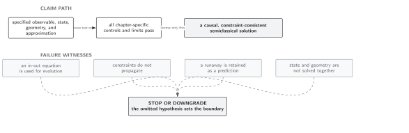
Validity boundary for mean black-hole evaporation. The map is schematic and not to scale; a controlled quasi-stationary interval licenses a mass-loss history only through the first failed adiabatic, curvature, state, or constraint check.

Domain and failure conditions

See the chapter domain and failure-conditions table. The mass law assumes a large nonextremal hole, collapse-compatible Unruh-like state, greybody-resolved asymptotic flux, slow evolution, low curvature in cutoff units, and a conserved completion of the stress tensor. It fails near the endpoint, at extremality or rapid evolution, for uncontrolled interior curvature, or when mean-field fluctuations are not small. No endpoint statement survives those failures.

Exercise

If $L_\infty=\alpha/M^2$, derive the adiabatic parameter $\lvert\dot\kappa\rvert/\kappa^2$ and show how it scales with $M$.

Solution

Since $\kappa=1/(4M)$ and $\dot M=-\alpha/M^2$,

$$\dot\kappa=-\frac{\dot M}{4M^2} =\frac{\alpha}{4M^4}, \qquad \frac{\lvert\dot\kappa\rvert}{\kappa^2} =\frac{\alpha/(4M^4)}{1/(16M^2)} =\frac{4\alpha}{M^2}.$$

It is small for $M^2\gg\alpha$ and grows as the mass decreases.

References

• del Río, A. “The Backreaction Problem for Black Holes in Semiclassical Gravity.” General Relativity and Gravitation 57 (2025): 30. DOI.
• del Río, A., and F. J. Marañón-González. “Black-Hole Evaporation from the Semiclassical Einstein Equations in 3+1 Dimensions.” arXiv preprint arXiv:2607.11737 (2026). arXiv.
• Page, D. N. “Particle Emission Rates from a Black Hole: Massless Particles from an Uncharged, Nonrotating Hole.” Physical Review D 13 (1976): 198–206. DOI.
• Unruh, W. G. “Notes on Black-Hole Evaporation.” Physical Review D 14 (1976): 870–892. DOI.