Tolman Redshift, KMS Structure, and Local Temperature

In stationary equilibrium, temperature redshifts with the norm of the timelike Killing field. A state that is KMS at inverse temperature $\beta$ with respect to one globally normalized Killing flow gives a static detector the local inverse temperature $\beta_{\mathrm{loc}}=\beta\sqrt{K^2}$. This is an operational equilibrium statement; a nonstationary trajectory or arbitrary rescaling of the generator without the corresponding $\beta$ transformation destroys the quoted scalar’s meaning.

Required background. Ground, KMS, and Symmetry-Selected States supplies the state condition; Unruh Effect and Uniformly Accelerated Detectors supplies detector detailed balance.

Helpful background. Thermal Density Operators and the KMS Condition supplies equilibrium notation; Conformal Transformations and Frame Changes supplies Weyl weights and their limits.

Killing time and proper time

Write a static metric as

$$\mathrm ds^2 = N(\mathbf x)^2\mathrm dt^2 -h_{ij}(\mathbf x)\mathrm dx^i\mathrm dx^j,$$

with $K=\partial_t$ and $N=\sqrt{K^\mu K_\mu}$. Along a static worldline,

$$\mathrm d\tau=N(\mathbf x)\,\mathrm dt.$$

Suppose the field state is KMS at inverse temperature $\beta$ with respect to $t$ translations. The imaginary shift $t\to t+i\beta$ becomes

$$\tau\to\tau+i\beta N.$$

Hence

$$\beta_{\mathrm{loc}}(\mathbf x) = \beta N(\mathbf x), \qquad T_{\mathrm{loc}}(\mathbf x) = \frac{T_K}{N(\mathbf x)},$$

or

$$T_{\mathrm{loc}}(\mathbf x)N(\mathbf x)=T_K.$$

This is the Tolman relation Tolman 1930, pp. 904–924.

A detector gap $\Omega$ is defined with respect to proper time. With respect to Killing time, the same transition has energy $N\Omega$. Detailed balance is therefore

$$\frac{\dot{\mathcal F}(+\Omega)} {\dot{\mathcal F}(-\Omega)} = e^{-\beta N\Omega} = e^{-\beta_{\mathrm{loc}}\Omega}.$$

The thermometer calibration and long-time approximation remain part of this operational inference.

First application: two radii in one static spacetime

Place identical static detectors at radii $r_1$ and $r_2$, with lapse values $N_1$ and $N_2$. Normalize the Killing generator once, for example by its norm in a specified asymptotic region. Then

$$\frac{T_{\mathrm{loc}}(r_1)} {T_{\mathrm{loc}}(r_2)} = \frac{N_2}{N_1},$$

while their proper gaps are both $\Omega$. Their Killing-energy gaps differ:

$$\Delta E_K(r_i)=N_i\Omega.$$

If both detectors reach the stationary detailed-balance regime, their excitation/de-excitation ratios are

$$R_i(\Omega)=e^{-\beta N_i\Omega}.$$

This is a reproducible comparison because the state, Killing normalization, proper gaps, trajectories, and protocol are common.

Near a Killing horizon $N\to0$, the Tolman temperature for a static detector can diverge. The proper acceleration needed to remain static also diverges. This does not state that a freely falling detector sees an arbitrarily hot local fluid; it concerns a singular family of static trajectories and a specified stationary state.

Generator and trajectory adversarial tests

Rescale the Killing vector,

$$K\longmapsto K'=cK.$$

Its parameter and Hamiltonian normalization change. The same KMS state is described with $\beta'=\beta/c$ so that $\beta K$ is invariant. Rescaling $K$ while leaving the numerical $\beta$ fixed changes the physical state specification; it is not a coordinate-invariant temperature comparison.

Next move a detector along a nonstationary trajectory. Its proper-time pullback need not be stationary or KMS, even though the global state remains KMS with respect to $K$. One can still compute a finite response, but one Tolman temperature is not licensed unless a controlled local-equilibrium approximation is separately shown.

Construction and failure maps

The structure map emphasizes that the normalized time flow and static worldline are chosen before detailed balance is interpreted as local temperature.

Tolman temperature is a calibrated KMS response with one fixed Killing normalization and static trajectory; the map is schematic and not to scale.

The failure map catches a rescaled generator or nonstationary trajectory before an unqualified local temperature is reported.

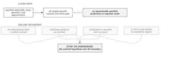
Only $T_{\mathrm{loc}}\sqrt{K^2}=T_K$ for the declared equilibrium flow and protocol is licensed; the map is schematic and not to scale.

Use the KMS comparison in Domain and failure conditions. This page’s decisive data are the normalized Killing generator, KMS parameter, lapse, proper detector gap, static trajectory, response window, and calibration range.

Check your understanding

If $N_1=1/2$ and $N_2=1$, what is $T_{\mathrm{loc}}(r_1)/T_{\mathrm{loc}}(r_2)$?

Solution

Tolman’s relation gives

$$\frac{T_{\mathrm{loc}}(r_1)} {T_{\mathrm{loc}}(r_2)} = \frac{N_2}{N_1}=2.$$

The detector deeper in the redshift well has twice the local equilibrium temperature for the same globally normalized KMS state.

Thermal equilibrium and hydrodynamics remain in Volume XI; horizon-specific KMS states and Hawking radiation belong to Chapter 6. This page does not identify every accelerated response with a scalar local temperature.

References

• Rudolf Haag, Nicolaas M. Hugenholtz, and Marinus Winnink, “On the Equilibrium States in Quantum Statistical Mechanics,” Communications in Mathematical Physics 5 (1967), 215–236, DOI.
• Richard C. Tolman, “On the Weight of Heat and Thermal Equilibrium in General Relativity,” Physical Review 35 (1930), 904–924, DOI.
• Richard C. Tolman and Paul Ehrenfest, “Temperature Equilibrium in a Static Gravitational Field,” Physical Review 36 (1930), 1791–1798, DOI.