Covariant Symplectic Structure and Conserved Inner Products

The field equation becomes quantizable only after its solution space is equipped with the correct conserved pairing. Real bosonic fields carry an antisymmetric symplectic form; complex or fermionic fields carry a conserved Hermitian form; gauge theories first carry a presymplectic form whose null directions must be quotiented or retained as boundary charges. Conservation makes these structures independent of the chosen Cauchy surface—unless flux escapes through a boundary.

Required background. Covariant Scalar Fields and Curvature Coupling supplies the model equation; Green Operators, Causal Propagators, and State-Dependent Two-Point Functions supplies the causal solution map; Presymplectic Systems and the Covariant Phase-Space Ambiguity Map supplies the variational construction.

Helpful background. Boundaries, Variations, and Well-Posed Actions explains surface terms; Canonical Quantization: Algebra, Representation, and State supplies the equal-time prototype.

The scalar symplectic current

Let $\phi_1$ and $\phi_2$ be real solutions of

$$P\phi=(\Box_g+m^2+\xi R)\phi=0.$$

The current

$$j^\mu(\phi_1,\phi_2) = \phi_1\nabla^\mu\phi_2 -\phi_2\nabla^\mu\phi_1$$

satisfies

$$\nabla_\mu j^\mu = \phi_1P\phi_2-\phi_2P\phi_1 =0.$$

On a spacelike Cauchy surface $\Sigma$ with future unit normal $n^\mu$,

$$\sigma_\Sigma(\phi_1,\phi_2) = \int_\Sigma \left( \phi_1n^\mu\nabla_\mu\phi_2 -\phi_2n^\mu\nabla_\mu\phi_1 \right)\mathrm d\Sigma .$$

For compactly supported Cauchy data, Stokes’ theorem between two Cauchy surfaces $\Sigma_1$ and $\Sigma_2$ gives

$$\sigma_{\Sigma_2}-\sigma_{\Sigma_1} = -\int_{\mathcal B}j^\mu s_\mu\,\mathrm d\mathcal B,$$

where $\mathcal B$ is any additional timelike or asymptotic boundary. With no such flux, the symplectic form is independent of the surface. This—not a coordinate-time Wronskian by itself—is the invariant conservation statement.

For complex scalar solutions, multiplication by $i$ converts the same current into the Klein–Gordon Hermitian form

$$(\phi_1,\phi_2)_{\mathrm{KG}} = i\int_\Sigma \left( \bar\phi_1n^\mu\nabla_\mu\phi_2 -(n^\mu\nabla_\mu\bar\phi_1)\phi_2 \right)\mathrm d\Sigma.$$

It is conserved but indefinite on the full complex solution space. Positivity arises only after choosing an appropriate positive-frequency subspace, which is extra representation data.

From test functions to phase space

For a formally self-adjoint Green-hyperbolic operator, the causal propagator maps compactly supported test functions to spacelike-compact solutions:

$$f\longmapsto Ef.$$

Functions differing by $Ph$ give the same solution, so the covariant phase space may be represented as

$$\mathcal E = C_0^\infty(M)\big/P C_0^\infty(M).$$

The antisymmetric bilinear form induced by $E$ is

$$\tau([f],[h]) = E(f,h).$$

With this chapter’s convention $E=G_{\mathrm{ret}}-G_{\mathrm{adv}}$, $\tau$ and the surface form differ by the corresponding fixed sign under the solution map; either representation is valid when used consistently. The quotient makes the equation of motion part of the phase-space definition rather than a later operator constraint.

The exact sequence identifying test functions modulo $P$ with spacelike-compact solutions, together with the induced symplectic form, is proved for Green-hyperbolic free fields in Bär, Ginoux, and Pfäffle 2007, §§3.4 and 4.3 and summarized for curved-spacetime QFT in Benini, Dappiaggi, and Hack 2013, §§2.2–2.3.

Fermions and gauge degeneracy

For Dirac solutions, the conserved current

$$j^\mu(\psi_1,\psi_2) = \bar\psi_1\gamma^\mu\psi_2$$

gives a positive Hermitian form on a Cauchy surface,

$$(\psi_1,\psi_2) = \int_\Sigma \bar\psi_1\gamma^\mu n_\mu\psi_2\,\mathrm d\Sigma.$$

This is the classical input to the CAR algebra. It should not be replaced by the indefinite bosonic Klein–Gordon form.

Gauge theories are different again. Their covariant two-form is generally presymplectic:

$$\Omega(\delta_\lambda A,\delta A)=0$$

for gauge transformations $\delta_\lambda A$ that vanish appropriately at the boundary. The physical bulk phase space quotients these null directions. Transformations with nonzero boundary charge are not null directions of the same physical problem and must not be discarded automatically. Reducible systems can also have cohomological degeneracies not generated by compactly supported gauge parameters.

First application: two Cauchy surfaces

Take a scalar solution on the slab bounded by Cauchy surfaces $\Sigma_1$ and $\Sigma_2$. Integrating the conserved current gives

$$0 = \int_{\mathcal V}\nabla_\mu j^\mu\,\mathrm d\mathrm{vol}_g = \sigma_{\Sigma_2} -\sigma_{\Sigma_1} +\int_{\mathcal B}j^\mu s_\mu\,\mathrm d\mathcal B.$$

If the spacetime has no timelike boundary and the data are spacelike compact, the last term vanishes and $\sigma_{\Sigma_2}=\sigma_{\Sigma_1}$. A canonical equal-time bracket computed on either surface therefore describes the same covariant phase space.

In a spatially flat FLRW spacetime, Fourier modes normalized by

$$a^{d-2} \left( \bar u_{\mathbf k}u'_{\mathbf k} -\bar u'_{\mathbf k}u_{\mathbf k} \right) =i$$

have a time-independent covariant Klein–Gordon normalization. Differentiating this expression and using the mode equation makes the Hubble-friction terms cancel. The factor $a^{d-2}$ is required by the surface measure and unit normal; omitting it creates a spurious time dependence.

Adversarial tests

Two changes reveal the limits of the conservation argument.

First, introduce a timelike boundary and impose no flux condition. Then

$$\sigma_{\Sigma_2}-\sigma_{\Sigma_1} = -\int_{\mathcal B}j^\mu s_\mu\,\mathrm d\mathcal B$$

need not vanish. The bulk equation still holds, yet the would-be phase-space form depends on the slice. A reflecting boundary condition, a compensating boundary degree of freedom, or an explicitly open-system interpretation is required.

Second, quantize an unreduced gauge potential as though its presymplectic form were nondegenerate. Pure-gauge directions then appear as zero-norm canonical coordinates, so inversion of the form and the resulting brackets are ill defined. Gauge fixing can facilitate calculation, but the physical phase space still requires the constraint and quotient or a cohomological BRST/BV construction.

The claim ceiling is therefore precise: current conservation gives slice independence only after support, boundary flux, and gauge degeneracy have been controlled.

Construction and failure maps

The construction map places the conserved solution-space pairing at the transition from classical propagation to quantization. The pairing must be nondegenerate after the correct gauge quotient.

Symplectic or Hermitian conservation links Cauchy evolution to the observable algebra only after boundary flux and gauge null directions are controlled; the map is schematic and not to scale.

The failure diagram should be read through Stokes’ theorem: nonzero timelike-boundary flux or an ignored presymplectic radical invalidates slice independence or invertibility.

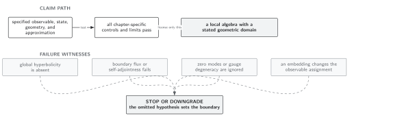
Current conservation licenses a Cauchy-surface-independent pairing only for the declared support and boundary conditions and after gauge reduction. Schematic and not to scale.

The chapter-wide comparison is under Domain and failure conditions. This page’s decisive checks are the on-shell current divergence, orientation of the surface normal, vanishing external flux, support decay, and nondegeneracy after constraints.

Check your understanding

Show that the FLRW Wronskian above is conserved for

$$u_{\mathbf k}'' +(d-2)\mathcal H u_{\mathbf k}' +\omega_{\mathbf k}^2u_{\mathbf k}=0.$$

Solution

Let $W=\bar u u'-\bar u'u$. The mode equation and its conjugate give

$$W'=-(d-2)\mathcal H W.$$

Because $(a^{d-2})'=(d-2)\mathcal H a^{d-2}$,

$$\left(a^{d-2}W\right)'=0.$$

Thus a normalization imposed on one Cauchy surface holds on every later surface so long as there is no boundary flux.

Covariant Algebraic Quantization and Fock Realizations promotes these pairings to CCR or CAR relations. General constrained reduction remains in Volume I, flat-space canonical brackets in Volume II, and theorem-level symplectic functors and completions in Volume XVI.

References

• Christian Bär, Nicolas Ginoux, and Frank Pfäffle, Wave Equations on Lorentzian Manifolds and Quantization, European Mathematical Society (2007), DOI, Open PDF, Chapter 4.
• Marco Benini, Claudio Dappiaggi, and Thomas-Paul Hack, “Quantum Field Theory on Curved Backgrounds: A Primer,” International Journal of Modern Physics A 28 (2013), 1330023, DOI, arXiv:1306.0527, §§2.2–2.3.
• Robert M. Wald, Quantum Field Theory in Curved Spacetime and Black Hole Thermodynamics, University of Chicago Press (1994), publisher record, Chapter 3.