Interacting Correlators and Curved-Space Time-Ordered Products

Interacting correlators on a curved background are built from time-ordered products of local functionals, not by multiplying singular propagators at coincidence. Causal ordering fixes these products away from partial diagonals; renormalization is the controlled extension to those diagonals. This separation identifies exactly where finite local ambiguities enter and keeps the choice of Hadamard state distinct from the operator definition.

Required background. Why local covariant renormalization supplies the structural axioms, and local composite-operator insertions supplies the functional derivatives used below.

Helpful background. The 1PI effective action organizes the same amplitudes after a Legendre transform, while scaling degree and extensions gives the distribution theorem underlying the diagonal step.

Time ordering before coincidence

For compactly supported local functionals $F_i$, write the formal local S-matrix

$$\mathcal S(F)=\sum_{n=0}^{\infty} \frac{1}{n!}\left(\frac{i}{\hbar}\right)^n T_n(F^{\otimes n}), \qquad T_0=\mathbf1.$$

The multilinear maps $T_n$ are symmetric, local and covariant, unitary in the appropriate formal sense, and causally factorizing. If the arguments are mutually noncoincident and causally ordered, lower-order products determine $T_n$. The remaining problem lies on unions of partial diagonals such as $x_1=x_2$ and on the total diagonal $x_1=\cdots=x_n$.

Choose a Hadamard two-point function to represent the free algebra. Wick expansion expresses a time-ordered product as operator monomials multiplied by numerical distributions made from the Feynman parametrix. For example, away from $x=y$,

$$T\!\left(\phi^4(x)\phi^4(y)\right) =\sum_{r=0}^{4} \binom{4}{r}^2r!\,[H_F(x,y)]^r :\!\phi^{4-r}(x)\phi^{4-r}(y)\!:\, .$$

The $r=2,3,4$ coefficients become progressively more singular as $y\to x$. Their products are well defined off the diagonal, where wavefront covectors cannot sum to zero in the forbidden way. The renormalization task is not to assign a pointwise value to $H_F^r$; it is to extend each coefficient distribution across the diagonal with the required scaling degree and covariance.

In four dimensions, the transverse codimension of the two-point diagonal is four. If a coefficient $t$ has scaling degree $s$, its degree of divergence is $\omega=s-4$. Extensions with the same scaling degree differ by derivatives of the delta distribution through order $\omega$:

$$t'-t=\sum_{|a|\leq\omega}C_a(x)\nabla^a\delta(x,y).$$

Local covariance restricts each $C_a$ to a local polynomial in curvature, masses, couplings, and background fields with the correct tensor type and dimension. The existence theorem is not a diagram-by-diagram appeal to a preferred coordinate system: Hollands and Wald construct local covariant time-ordered products and obtain their scaling expansion near the diagonal (Hollands and Wald 2002, Theorems 4.1–5.2).

From products to correlators

Let

$$V(g)=-\int_M d^4x\sqrt{-g}\, g(x)\frac{\lambda}{4!}\phi^4(x),$$

with $g\in C_c^\infty(M)$. The interacting version of an observable $F$ is the Bogoliubov derivative

$$R_V(F)=\left.\frac{\hbar}{i}\frac{d}{dt}\right|_{t=0} \mathcal S(V)^{-1}\mathcal S(V+tF).$$

Expanding this expression yields retarded products. A Hadamard state $\omega$ then gives an interacting correlation functional $\omega(R_V(F_1)\cdots R_V(F_n))$. Two choices enter at different levels:

1. changing $T_n$ by an allowed finite local map changes the renormalization prescription and is compensated by counterterms and operator redefinitions;
2. changing $\omega$ changes the smooth state-dependent parts of the correlator without changing the locally covariant product.

Interacting correlators remain formal power series in $\lambda$ unless a separate summability or convergence statement is made.

The construction map places diagonal extension immediately before causal factorization. For the four-point example below, inspect that junction: the coefficient distributions must be extended first, and only then can their local S-matrix satisfy the causal identities.

Time-ordered products are the ultraviolet input to the interacting construction. This schematic, not-to-scale map emphasizes that diagonal extension is controlled by locality, scaling, covariance, and Ward identities before local observables are claimed.

The failure map isolates the adversarial mistake on this page: an undefined product is not repaired by formally covariant notation. Failure of the wavefront or extension check stops the claim at separated points.

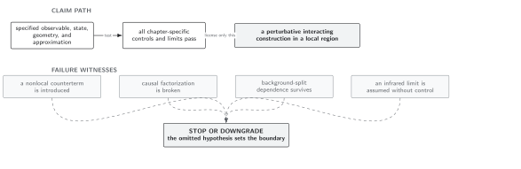
Claim boundary for singular products. The map is schematic and not to scale; a failed distributional product requires a downgrade to its valid noncoincident domain rather than an arbitrary coincident value.

Application: the second-order scalar four-point function

Take four distinct external points $x_1,\ldots,x_4$ and the connected contribution with two interaction vertices $u,v$. Before extension to $u=v$, a representative Wick-contraction topology has coefficient

$$G_F(x_1,u)G_F(x_2,u) [G_F(u,v)]^2 G_F(x_3,v)G_F(x_4,v),$$

plus permutations and topologies with tadpoles. The second-order term is

$$G^{(4)}_{(2),c} =\frac{1}{2}\left(-\frac{i\lambda}{4!\hbar}\right)^2 \int d\mu_g(u)d\mu_g(v)\,g(u)g(v) \,\mathcal C(x_1,\ldots,x_4;u,v),$$

where $\mathcal C$ is the sum with its Wick combinatorics. This formula is meaningful only after specifying extensions on all relevant strata.

The diagonal ambiguities at this order are classified by the local operators allowed in the four-dimensional action and insertions:

• on the vertex diagonal $u=v$: $\phi^4$, $\phi^2$, $(\nabla\phi)^2$, $R\phi^2$, and identity operators $1,R,R^2,R_{\mu\nu}R^{\mu\nu},R_{\mu\nu\rho\sigma}R^{\mu\nu\rho\sigma},\Box R$, with coefficients carrying the necessary powers of $m$;
• on a vertex–external-point diagonal: local field and composite-insertion renormalizations, including contact terms proportional to delta distributions and their allowed derivatives;
• where several external points coincide: additional composite-product contact terms, relevant only if the four-point distribution is pulled back to that diagonal.

Modulo integrations by parts and the field equation, one may reduce this list to an independent basis. The list is broader than the superficially divergent four-point graph alone because the complete second-order time-ordered product must also renormalize its lower-point contractions. Numerical coefficients depend on the chosen extension; the operator basis does not.

Adversarial test: the undefined square

Suppose one writes $G_F(u,v)^2$ as an ordinary function and immediately sets $v=u$. The Feynman propagator is a distribution singular on the null cone and at coincidence. Its pointwise square at the diagonal has no intrinsic meaning; in local coordinates its leading behavior resembles $(\sigma+i0)^{-2}$, whose extension is logarithmically ambiguous. Formal covariance of the symbols does not repair the missing distribution.

The correct sequence is: restrict to the complement of the diagonal, verify the microlocal product there, determine scaling degree, extend locally and covariantly, and record the finite delta-supported freedom. If wavefront compatibility already fails off the diagonal for a proposed pullback, even this extension step is unavailable. The surviving object is then only the correlator smeared on a domain avoiding the forbidden coincidence.

Domain and failure conditions

Use the chapter domain and failure-conditions table to place this method. The data are the free Hadamard kernel, local vertices, every partial diagonal, perturbative order, and the scaling degree of each numerical distribution. They license a renormalized time-ordered product only after microlocal multiplication off the diagonals and local covariant extension onto them. The decisive checks are causal factorization and extension ambiguity confined to the permitted delta-supported basis. If either fails, the result is only a separated-point or more narrowly smeared distribution; the handoff to counterterm classification is valid only for extensions that pass those checks.

Checks and limits

• Causal check: when all vertices of one factor are later than those of another, $T$ must factor with the later factor on the left.
• Flat limit: in a geodesically convex region with vanishing curvature, the local singular part reduces to the Minkowski extension in matching coordinates and scheme.
• State check: replacing one Hadamard two-point function by another changes Wick contractions through a smooth kernel; it cannot change which ultraviolet diagonal counterterms are allowed.
• Support check: compact $g$ makes every perturbative coefficient a well-defined smeared distribution; $g\to1$ is a separate infrared problem.

Exercise

In four dimensions the leading singularity of $H_F(x,y)$ has scaling degree $2$ in the relative coordinate. What is the finite extension freedom of $H_F^2$ at $x=y$?

Solution

The square has scaling degree $4$, equal to the diagonal codimension. Thus $\omega=0$, so two extensions differ only by $C(x)\delta(x,y)$, with no derivatives of the delta distribution. Covariance and dimension restrict the scalar coefficient $C$ to a dimensionless function of dimensionless couplings; factors such as $m^2$ or $R$ would have too high a dimension for this coefficient. More singular graphs can admit derivative and curvature-dependent terms.

Handoff

Diagonal extension tells us where the ambiguity is supported. The next page classifies the local matter and curvature operators that can occupy that support and shows how composite insertions mix.

References

• Brunetti, Romeo, and Klaus Fredenhagen. “Microlocal Analysis and Interacting Quantum Field Theories: Renormalization on Physical Backgrounds.” Communications in Mathematical Physics 208 (2000): 623–661. doi:10.1007/s002200050004.
• Hollands, Stefan, and Robert M. Wald. “Existence of Local Covariant Time Ordered Products of Quantum Fields in Curved Spacetime.” Communications in Mathematical Physics 231 (2002): 309–345. doi:10.1007/s00220-002-0719-y.
• Hollands, Stefan, and Robert M. Wald. “Quantum Fields in Curved Spacetime.” Physics Reports 574 (2015): 1–35. doi:10.1016/j.physrep.2015.02.001.