Mode-Sum and Numerical Renormalization

Mode-sum renormalization turns a divergent spectral representation into a local observable by subtracting an analytically derived high-mode expansion, summing the regular remainder, and restoring the subtracted finite part. A converged cutoff sum is not sufficient: the asymptotic coefficients, tail bound, low modes, precision loss, and independent scheme check must all be controlled.

Required background. Curved-Space Renormalization Schemes: Domains and Translation supplies the local subtraction; Vacuum Polarization and Curved-Space Casimir Effects supplies the relative observables; Spectra, Resolvents, and Functional Calculus supplies the spectral decomposition.

Helpful background. Asymptotic Scales, Remainders, and Uniformity supplies remainder logic; Special Functions: Equations and Boundary Data supports stable mode evaluation.

Analytic subtraction before numerical summation

Suppose a point-split observable has the regulated representation

$$\mathcal O(\varepsilon;x) = \sum_{\ell=0}^{\infty}d_\ell\, F_\ell(\varepsilon;x),$$

where $\varepsilon$ is a temporal, radial, or angular split. Apply the same mode transform to the Hadamard or DeWitt–Schwinger counterterm:

$$H_{\mathcal O}(\varepsilon;x) = \sum_{\ell=0}^{\infty}d_\ell\, S_\ell(\varepsilon;x).$$

Then

$$\langle\mathcal O(x)\rangle_{\mathrm{ren}} = \sum_{\ell=0}^{\infty}d_\ell \left[F_\ell(0;x)-S_\ell(0;x)\right] +\mathcal O_{\mathrm{an}}(x),$$

where $\mathcal O_{\mathrm{an}}$ contains the analytically restored local part and the declared finite prescription. The split is kept nonzero until the mode transform and distributional terms have been handled. This is the numerical form of point splitting, not a separate definition.

Let $L=\ell+\tfrac12$. After subtraction through order $K$, suppose the summand has

$$r_\ell(x) = d_\ell[F_\ell-S_\ell] = \frac{a_p(x)}{L^p} +O(L^{-p-2}), \qquad p>1.$$

If $|r_\ell|\le C L^{-p}$ beyond $L_*$, the uncomputed tail obeys

$$\left|\sum_{\ell>\ell_{\max}}r_\ell\right| \le \frac{C}{p-1} \left(\ell_{\max}+\frac12\right)^{1-p}.$$

This bound must be combined with ODE, quadrature, and roundoff errors. The analytic coefficients come from the local parametrix or a controlled WKB recursion; they are not inferred solely by fitting the available modes.

First application: static spherical field square

For

$$\mathrm ds^2=f(r)\,\mathrm dt^2-h(r)\,\mathrm dr^2-r^2\mathrm d\Omega_2^2,$$

decompose a Hadamard scalar two-point function into frequency and angular modes. At fixed $r$, the regulated field square can be organized as

$$\langle\phi^2(r)\rangle_{\mathrm{ren}} = \sum_{\ell=0}^{\ell_{\max}} \left[\mathcal F_\ell(r)-\mathcal S_\ell^{(K)}(r)\right] +\mathcal T_{\ell_{\max}}^{(K)}(r) +\mathcal A^{(K)}(r).$$

Here $\mathcal F_\ell$ includes the frequency integral and degeneracy, $\mathcal S_\ell^{(K)}$ is the analytic large-$L$ subtraction, $\mathcal T$ is the quantified residual tail, and $\mathcal A$ restores the finite local terms. Levi and Ori develop this point-splitting-to-mode-sum construction for stationary black-hole backgrounds Levi and Ori 2015, §§II–IV, pp. 3–15 of the arXiv PDF.

A reproducible calculation performs these separate tests:

• increase frequency range and quadrature precision at fixed $\ell_{\max}$;
• increase $\ell_{\max}$ at fixed subtraction order;
• increase $K$ and verify the predicted change in the tail power;
• recompute sensitive low modes with independent initial data or higher precision;
• verify that the difference between two subtraction prescriptions is the predicted local finite term;
• compare selected points with an independent point-splitting, Euclidean, or high-precision fixture.

Cancellation can destroy digits when $\mathcal F_\ell$ and $\mathcal S_\ell$ are individually large. If their scale is $M_\ell$ and the remainder is $r_\ell$, the calculation needs substantially more than

$$\log_{10}\left|\frac{M_\ell}{r_\ell}\right|$$

guard digits before the subtraction. A stable plateau under $\ell_{\max}$ is meaningless if every remainder has already lost its significant digits.

The stress tensor needs more subtraction orders and derivative data than $\phi^2$. Anderson, Hiscock, and Samuel give a systematic analytic–numerical decomposition for static spherical stress tensors Anderson, Hiscock, and Samuel 1995, §§II–IV, pp. 4339–4351. Finite $\phi^2$ convergence therefore does not certify the stress calculation.

Adversarial fitted-tail test

Fit the last ten computed modes to $a/L^p+b/L^{p+2}$ and extrapolate. If the fitted window has not entered the asymptotic regime, omitted logarithms or lower powers can mimic an excellent residual while biasing the infinite tail. Shift the fit window, add the analytically predicted next basis function, and compare with a coefficient derived from the parametrix.

If the inferred observable moves beyond the combined numerical error, the fit was diagnostic rather than evidential. The strongest surviving claim is the finite cutoff result plus an unresolved tail. An infinite-sum value requires analytic asymptotics or a validated enclosure.

Numerical and failure maps

The structure map places the analytic counterterm beside the raw modes and reunites them only after the residual tail is controlled.

Cutoff convergence, subtraction order, and scheme translation are separate controls in a numerical local observable; the map is schematic and not to scale.

The failure map highlights false plateaus from empirical tails, precision loss, missing low modes, and inconsistent local terms.

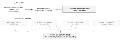
A reliable infinite sum needs analytic large-mode control and an independent local-covariant check; the map is schematic and not to scale.

Use Domain and failure conditions. Report state and boundary conditions, split direction, mode normalization, subtraction order, finite prescription, cutoff sequence, tail model and bound, precision, low-mode treatment, Ward residual, and independent fixture.

Check your understanding

If the subtracted summand behaves as $r_\ell\sim a/L^4$, how should its remaining tail scale?

Solution

The integral test gives $\sum_{\ell>\ell_{\max}}L^{-4}=O(L_{\max}^{-3})$. A log–log plot of the cutoff error should approach slope $-3$ before the stated tail law is trusted.

Geometric Discretization and Continuum Checks treats mesh refinement. Independent implementations may execute these calculations, but the page-level result remains conditional on the analytic and numerical checks above.

References

• Paul R. Anderson, William A. Hiscock, and David A. Samuel, “Stress-Energy Tensor of Quantized Scalar Fields in Static Spherically Symmetric Spacetimes,” Physical Review D 51 (1995), 4337–4358, DOI.
• Adam Levi and Amos Ori, “Pragmatic Mode-Sum Regularization Method for Semiclassical Black-Hole Spacetimes,” Physical Review D 91 (2015), 104028, DOI, arXiv:1503.02810.