Hadamard Admissibility and the Two-Point Wavefront Criterion

The microlocal Hadamard condition records both where a two-point distribution is singular and which cotangent directions carry each singularity. For a real scalar Klein–Gordon field on a four-dimensional, boundaryless, globally hyperbolic spacetime, it is equivalent to the familiar local Hadamard expansion. This is the right ultraviolet condition for local observables, but it neither selects a preferred state nor replaces the field equation, commutation relation, or positivity.

Required background. Hadamard Parametrix and Short-Distance Structure gives the local singular form. Singular Support and Wavefront Sets defines directional singularity. Products, Scaling Degree, and Distribution Extensions explains why wavefront information controls products.

Helpful background. Operator Algebras and Positive Functionals keeps admissibility distinct from state positivity. Microcausality and Relativistic Compatibility supplies the causal interpretation.

How to read a wavefront-set point

For an ordinary function, a singular point is a point of spacetime. For a distribution $u$, a wavefront-set element $(x,k)$ carries two pieces of information:

• $x$ is the base point at which smoothness fails;
• $k\ne0$ is a cotangent direction in which rapid Fourier decay fails.

The direction is conic: if $(x,k)\in\operatorname{WF}(u)$, then $(x,ak)$ is also present for every $a>0$. Its magnitude therefore has no invariant meaning. Its ray and time orientation do.

A two-point distribution lives on $M\times M$, so one wavefront element has two slots,

$$(x,k;x',q)\in \dot T^*(M\times M).$$

The semicolon merely separates the two copies of spacetime. It is not a causal arrow. The dot removes only the zero covector of the product bundle, so $(k,q)$ cannot have both entries zero; a general bidistribution can still have a partial-zero element $(0,q)$ or $(k,0)$. The Hadamard relation defined below has neither kind because its two nonzero covectors are linked by parallel transport.

The Hadamard relation

Let

$$P_\xi=\Box+m^2+\xi R$$

with real $m^2$ and $\xi$. Assume the metric and coefficients are smooth, the spacetime is oriented and time oriented, and there is no boundary. Write $k\triangleright0$ when the nonzero covector $k$ is future directed; with the $(+---)$ metric convention, $k(v)>0$ for every future-directed timelike vector $v$.

We write

$$(x,k)\sim(x',k')$$

when there is a null geodesic $\gamma$ through $x$ and $x'$, the covector $k\in T_x^*M\setminus\{0\}$ is null with $k^\sharp$ tangent to $\gamma$ at $x$, and $k'$ is the parallel transport of $k$ along $\gamma$. For $x=x'$, the standard zero-length case retains a chosen nonzero null direction and has $k'=k$. Thus the covector direction is tied to the same null ray that joins the base points; merely transporting an arbitrary covector between two null-related points is not enough. The Hadamard cone is

$$\mathcal C^+ = \left\{ (x,k;x',-k'): (x,k)\sim(x',k'),\quad k\triangleright0 \right\}.$$

For a Hadamard two-point function,

$$\boxed{\operatorname{WF}(\omega_2)=\mathcal C^+.}$$

This compact formula says four things at once: the singular directions are null; the two base points are joined by the corresponding null geodesic; the covector is parallel transported between them; and the first slot uses the future branch while the second slot carries its negative. The equivalence with the four-dimensional local Hadamard form is Radzikowski 1996, Theorem 5.1, pp. 545–547; a modern formulation and explanation appear in Khavkine and Moretti 2015, Theorem 9, pp. 47–49 (Open PDF).

The diagram makes the signs and the two different spaces explicit. Follow the solid null ray from $x$ to $x'$: $k'$ is the transported geometric covector, whereas the covector entered in the second distribution slot is $-k'$.

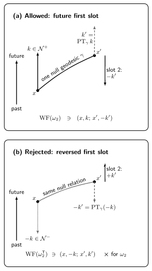
Allowed Hadamard pairing and its orientation control. The nonzero null covector $k$ has $k^\sharp$ tangent to the same null geodesic that joins the base points. Parallel transport relates $k$ to $k'$, but the product-cotangent element is $(x,k;x',-k')$. A past-directed first covector belongs to the transposed cone, not to $\operatorname{WF}(\omega_2)$. Original schematic; not to scale. Semantic description (JSON).

Why the second covector has a minus sign

In Minkowski spacetime, a translation-invariant kernel depends on $z=x-x'$. If a singular Fourier direction is $p$ in $z$, changing $x$ changes $z$ by the same amount, while changing $x'$ changes it by the opposite amount. The corresponding product-cotangent direction is therefore

$$(x,p;x',-p).$$

Curvature changes straight null lines into null geodesics and replaces equality of covectors by parallel transport. It does not change this slot sign.

The same fact is encoded by the commutator. With the site convention

$$E=G_{\mathrm{ret}}-G_{\mathrm{adv}}, \qquad \omega_2-\omega_2^{\mathsf T}=-iE,$$

the transpose $\omega_2^{\mathsf T}(x,x')=\omega_2(x',x)$ carries the opposite cone $\mathcal C^-$. The commutator contains both orientations, while a positive-frequency two-point function contains only the future orientation in its first slot.

Why equality is stronger than inclusion

One sometimes meets a cone condition written only as $\operatorname{WF}(w)\subset\mathcal C^+$. That is a useful upper bound for a candidate distribution, but by itself it is too weak: every smooth kernel, including zero, obeys it.

For a genuine Klein–Gordon two-point function, the field equation confines singularities to the characteristic cone and the fixed antisymmetric part supplies the full singular content of $E$. Since

$$\operatorname{WF}(E)=\mathcal C^+\cup\mathcal C^-,$$

the commutator and the one-sided inclusion force the exact equality. This reasoning depends on the bisolution and commutator hypotheses. It must not be applied to an arbitrary distribution.

The logical jobs are distinct:

Condition	What it establishes	What it does not establish
$P_{\xi,x}\omega_2=P_{\xi,x'}\omega_2=0$	Free-field dynamics in both slots	Positivity or time orientation
$\omega_2-\omega_2^{\mathsf T}=-iE$	Canonical antisymmetric part	The positive symmetric part
$\operatorname{WF}(\omega_2)=\mathcal C^+$	Hadamard ultraviolet singularity	A preferred vacuum
$\omega_2(\bar f,f)\ge0$	Positive type	Hadamard regularity
Hermiticity and all four rows together	A Hadamard state two-point function	Uniqueness of the state

Minkowski vacuum: extracting the orientation

In four-dimensional Minkowski spacetime,

$$\omega_2(x,x') = \int\frac{\mathrm d^3\mathbf p}{(2\pi)^3 2\omega_{\mathbf p}} \exp\!\left[-i\omega_{\mathbf p}(t-t') +i\mathbf p\cdot(\mathbf x-\mathbf x')\right], \qquad \omega_{\mathbf p}=\sqrt{\lvert\mathbf p\rvert^2+m^2}.$$

Use the Fourier-transform convention with testing phase $e^{+ik\cdot x}$. The spectral support of the first variable is then the positive-energy mass shell, whose covector components are

$$p_a=(\omega_{\mathbf p},-\mathbf p), \qquad p_0>0.$$

Wavefront sets retain only conic high-frequency directions. For fixed nonzero $\mathbf q$,

$$\frac{1}{\lambda} (\omega_{\lambda\mathbf q},-\lambda\mathbf q) \longrightarrow (\lvert\mathbf q\rvert,-\mathbf q) \quad(\lambda\to\infty),$$

which is future directed and null. Translation invariance supplies its negative in the second slot. The mass affects the smooth, finite-frequency content but not this ultraviolet cone.

Transposing the kernel changes $x-x'$ to $x'-x$ and hence gives $\mathcal C^-$. Both kernels have the same singular support—null-related pairs—but their wavefront orientations differ. This is precisely the information singular support forgets.

Same wavefront set, different states

The criterion deliberately leaves the smooth state-dependent remainder free. Let $u$ be a real smooth solution of $P_\xi u=0$ and let $\lambda\ge0$. Starting from any Hadamard state two-point function, define

$$\omega_2^{(\lambda)}(x,x') = \omega_2(x,x')+\lambda u(x)u(x').$$

The added term is a smooth symmetric bisolution, so it changes neither the commutator nor the wavefront set. It also preserves positivity because

$$\omega_2^{(\lambda)}(\bar f,f) = \omega_2(\bar f,f)+\lambda\lvert u(f)\rvert^2 \ge0.$$

Thus $\omega_2$ and $\omega_2^{(\lambda)}$ are distinct Hadamard state two-point functions with identical wavefront sets. Under the same point-splitting prescription their Wick-square expectations differ exactly by

$$\langle{:}\Phi^2(x){:}\rangle_{\lambda} - \langle{:}\Phi^2(x){:}\rangle_{0} =\lambda u(x)^2.$$

Derivatives of the same smooth remainder change stress-tensor expectations. Microlocal admissibility therefore fixes the universal singular class, not the physical state within that class.

Products, limitations, and failure tests

The one-sided cone makes specific free-field products well defined. For example, when powers of the same Hadamard kernel are formed on $M\times M$, sums of their first-slot covectors remain future directed and cannot cancel to zero; the second-slot sums remain past directed. This does not license arbitrary products: combining a kernel with its transpose can present opposite covectors and must be checked separately against Hörmander’s zero-sum criterion. Local Wick powers still require subtraction of the Hadamard parametrix before taking coincidence limits. The higher-point graph condition and its use in Wick-polynomial constructions are developed by Brunetti, Fredenhagen, and Köhler 1996, §§2–4.

The scalar equality above has a declared domain. A timelike boundary requires boundary conditions and may introduce reflected wavefront branches. Gauge fields require constraints or a subsidiary construction. A non-globally-hyperbolic region needs additional input, and a finite-order adiabatic state may satisfy only a Sobolev version of the regularity condition. In each case the remedy is a field- and domain-specific theorem, not a silent reuse of the scalar formula.

Microlocal and algebraic controls must both pass. A kernel can have the correct cone and fail positivity, or be positive while carrying a forbidden wavefront direction. The logical table separates those tests, while the pairing figure makes the geometric sign control explicit.

For neighboring state claims and their exact domains, see Domain and failure conditions.

Common pitfalls

Reading $-k'$ as backward transport. Parallel transport sends $k$ to $k'$. The minus sign is attached only when that transported covector is placed in the second distribution slot.

Calling every future-cone distribution a state. The cone condition does not imply the field equation, Hermiticity, the canonical commutator, or positive type. Check those conditions separately.

Treating mass-shell momenta as the wavefront cone. Massive Fourier modes lie on a timelike mass shell at finite momentum. Their conic ultraviolet limit is null, which is why the principal symbol—not the mass—determines the wavefront directions.

Exercises

1. Opposite slot covectors. Let $K(x,x')=F(x-x')$. Show that every wavefront element of $K$ has the form $(x,k;x',-k)$.

Solution

Introduce $z=x-x'$. A variation $(\delta x,\delta x')$ changes $z$ by $\delta z=\delta x-\delta x'$. Pulling a covector $k$ on the $z$ space back through this map gives

$$k(\delta z)=k(\delta x)-k(\delta x'),$$

so the product-space covector is $(k,-k)$. The same pullback rule applies to the wavefront set whenever the pullback is defined.

2. Ultraviolet null limit. Verify that the positive-energy massive momentum in the Minkowski integral approaches a null covector after conic rescaling.

Solution

For $\mathbf p=\lambda\mathbf q$,

$$\frac{\omega_{\lambda\mathbf q}}{\lambda} = \sqrt{\lvert\mathbf q\rvert^2+\frac{m^2}{\lambda^2}} \longrightarrow\lvert\mathbf q\rvert.$$

Hence $p_a/\lambda\to(\lvert\mathbf q\rvert,-\mathbf q)$, whose squared norm in the $(+---)$ convention is zero and whose time component is positive.

3. Transpose test. Determine the wavefront set and antisymmetric part of $\omega_2^{\mathsf T}$.

Solution

Swapping the variables maps $(x,k;x',-k')$ to $(x',-k';x,k)$, so the first covector is past directed and $\operatorname{WF}(\omega_2^{\mathsf T})=\mathcal C^-$. Moreover,

$$\omega_2^{\mathsf T}-\omega_2=+iE.$$

It therefore has the opposite canonical commutator and is not a state two-point function for the same algebra convention.

4. A family the cone cannot distinguish. Check every two-point condition for $\omega_2^{(\lambda)}=\omega_2+\lambda u\otimes u$ with real smooth $P_\xi u=0$ and $\lambda\ge0$.

Solution

The added kernel is smooth, symmetric, Hermitian, and a bisolution. It therefore leaves the wavefront set and antisymmetric part unchanged. Its quadratic form is $\lambda\lvert u(f)\rvert^2\ge0$, so positivity is preserved. Unless $\lambda=0$ or $u=0$, the smooth remainder and local expectation values change. The Hadamard cone therefore classifies ultraviolet behavior without selecting a unique state.

Handoffs

Propagation of the Hadamard Property explains why the condition extends from a complete Cauchy neighborhood. Hadamard States for Fermion and Gauge Fields adapts it to other field complexes. The proof and precise bundle-valued extensions continue in Hadamard States and the Wavefront-Set Characterization.

References

• Brunetti, Romeo, Klaus Fredenhagen, and Michael Köhler. “The Microlocal Spectrum Condition and Wick Polynomials of Free Fields on Curved Spacetimes.” Communications in Mathematical Physics 180 (1996): 633–652. DOI. Open PDF.
• Khavkine, Igor, and Valter Moretti. “Algebraic QFT in Curved Spacetime and Quasifree Hadamard States: An Introduction.” In Advances in Algebraic Quantum Field Theory, 191–251. Cham: Springer, 2015. DOI. Open PDF.
• Radzikowski, Marek J. “Micro-Local Approach to the Hadamard Condition in Quantum Field Theory on Curved Space-Time.” Communications in Mathematical Physics 179 (1996): 529–553. DOI.