Gauge Fields, Gauge Fixing, and Ghosts on Curved Backgrounds

Gauge symmetry makes the potential equation degenerate: configurations related by a gauge transformation represent the same physical field. On a curved background, gauge fixing converts the differential expression into a Green-hyperbolic operator, but the resulting potential propagator depends on the gauge parameter. Physical conclusions must be expressed through gauge-invariant observables or BRST cohomology, with residual transformations, zero modes, topology, and boundary data treated separately.

Required background. Curved Spacetimes, Cauchy Surfaces, and Global Hyperbolicity supplies the causal setting; The Free Maxwell Field and Gauge Redundancy supplies the constraint structure; Vector, Principal, and Associated Bundles supplies the geometric setting for connections.

Helpful background. Presymplectic Systems and the Covariant Phase-Space Ambiguity Map explains gauge degeneracy; The Faddeev–Popov Construction supplies the ghost determinant.

Maxwell fields before gauge fixing

For an Abelian potential $A_\mu$,

$$F_{\mu\nu}=2\nabla_{[\mu}A_{\nu]}, \qquad A_\mu\longmapsto A_\mu+\nabla_\mu\lambda,$$

and

$$S[A] = -\frac14 \int_M\mathrm d^dx\,\sqrt{-g}\, F_{\mu\nu}F^{\mu\nu}.$$

The equation of motion is

$$\nabla_\mu F^{\mu\nu}=0.$$

In terms of the potential,

$$\Box_gA^\nu-\nabla^\nu(\nabla_\mu A^\mu)-R^\nu{}_\mu A^\mu=0$$

for the site curvature convention. Its principal symbol has the null vector $k_\mu$, reflecting gauge degeneracy. Consequently, the unfixed potential operator has no inverse on the full space of one-forms.

The gauge-invariant local field is $F_{\mu\nu}$. Wilson loops and fluxes add global observables when topology permits. Charged fields, dressings, and non-Abelian self-interactions require additional structure and are not inferred from the free Maxwell system.

Hyperbolic gauge fixing and ghosts

Add the covariant gauge-fixing term

$$S_{\mathrm{gf}} = -\frac{1}{2\alpha} \int_M\mathrm d^dx\,\sqrt{-g}\, (\nabla_\mu A^\mu)^2.$$

For $\alpha=1$, the potential satisfies the normally hyperbolic equation

$$P^\nu{}_\mu A^\mu = \left( \delta^\nu{}_\mu\Box_g-R^\nu{}_\mu \right)A^\mu =0.$$

Other values of $\alpha$ change the longitudinal part of the potential propagator. In Abelian theory, the Faddeev–Popov operator is the scalar $\Box_g$; the ghosts are free and decouple from local field-strength correlators in ordinary perturbation theory. Their determinant and zero modes still matter in functional measures and finite-volume or boundary problems.

BRST notation makes the physical criterion concise:

$$sA=\mathrm dc, \qquad sc=0, \qquad s\bar c=B, \qquad sB=0.$$

Physical observables are BRST-closed modulo BRST-exact terms, subject to anomaly and boundary qualifications. The general BRST/BV construction belongs to Volume III.

First application: an ultrastatic background

Let

$$M=\mathbb R\times\Sigma, \qquad g=\mathrm dt^2-h_{ij}(\mathbf x)\mathrm dx^i\mathrm dx^j,$$

with $\Sigma$ complete and with no boundary. In Feynman gauge, the Green operator of $P^\nu{}_\mu$ defines a potential two-point function $W_{\mu\nu'}(x,x')$ after a state is chosen. Changing $\alpha$ changes $W_{\mu\nu'}$ by longitudinal terms of the form

$$\nabla_\mu\nabla_{\nu'}H(x,x').$$

The field-strength two-point function is obtained by antisymmetric differentiation:

$$\left\langle F_{\mu\nu}(x)F_{\rho'\sigma'}(x') \right\rangle = 4\nabla_{[\mu}\nabla_{[\rho'} W_{\nu]\sigma']}(x,x').$$

The added longitudinal term drops out because covariant derivatives commute on scalars before antisymmetrization. Thus the potential correlator is gauge dependent while the local field-strength correlator is unchanged. This is a direct gauge-independence check, not a claim that every nonlocal or boundary observable is independent of gauge fixing.

Residual transformations, zero modes, and boundaries

Lorenz gauge leaves residual transformations satisfying

$$\Box_g\lambda=0.$$

On a compact spatial slice, constant modes and harmonic one-forms require separate treatment. Dividing by the local gauge volume does not automatically remove global holonomies or flux sectors. Fewster and Lang show that the universal Maxwell theory on arbitrary topology can acquire nontrivial radicals classically and central elements quantum mechanically; a reduced theory restores the desired locality properties by removing the appropriate degeneracies Fewster and Lang 2015, §§3–6.

A boundary adds two further choices: which gauge transformations are allowed at the boundary and which flux condition makes the variational principle and symplectic form well defined. A transformation that does not vanish at the boundary can carry a charge rather than represent a redundancy. Imposing $A_\parallel=0$, fixing electric flux, or adding boundary degrees of freedom therefore gives physically different theories.

The adversarial test is immediate:

1. vary $\alpha$ and verify that the claimed quantity is unchanged;
2. add a residual zero mode and check whether the gauge condition fixes it;
3. change the boundary condition and recompute the symplectic flux;
4. express the final claim in terms of $F$, a Wilson observable, or a BRST cohomology class.

If a result fails the first test, it is gauge dependent. If the operator has unremoved zero modes, an advertised inverse is undefined until a domain or quotient is supplied.

Construction and failure maps

The first map should be read with “symplectic or gauge reduction” emphasized. Gauge fixing makes a useful hyperbolic representative, while reduction or BRST cohomology determines which later algebraic elements are physical.

Gauge fixing supports propagation, but gauge reduction, topology, and boundary charges determine the physical algebra; the map is schematic and not to scale.

In the failure map, inspect the zero-mode and boundary witnesses. Gauge-parameter independence of $F_{\mu\nu}$ is necessary but does not settle residual modes, holonomies, or charged boundary transformations.

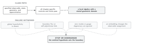
Only gauge-invariant or cohomological observables with controlled zero modes and boundary data are licensed as physical conclusions; the map is schematic and not to scale.

The chapter comparison appears under Domain and failure conditions. For a vector field, check the constraint, gauge-fixed operator, residual kernel, ghost complex, gauge-parameter independence, topology, and boundary charge assignment before interpreting a correlator.

References

• Marco Benini, Claudio Dappiaggi, and Alexander Schenkel, “Quantized Abelian Principal Connections on Lorentzian Manifolds,” Communications in Mathematical Physics 330 (2014), 123–152, DOI, arXiv:1303.2515.
• Christopher J. Fewster and Benjamin Lang, “Dynamical Locality of the Free Maxwell Field,” Annales Henri Poincaré 17 (2016), 401–436, DOI, arXiv:1403.7083.
• Stefan Hollands and Robert M. Wald, “Quantum Fields in Curved Spacetime,” Physics Reports 574 (2015), 1–35, DOI, Open PDF, §3.3.