

Power Spectra, Horizon Crossing, and Freeze-Out
A power spectrum is a late-time two-point function, whereas “horizon crossing” names an intermediate epoch. Replacing evolution by evaluation at is accurate only when background parameters vary slowly and the relevant long-wavelength mode rapidly approaches a constant attractor solution.
Required background. Mukhanov–Sasaki scalar modes supplies scalar normalization; tensor modes supplies both helicities; and vacuum choice and initial-state effects supplies the state condition.
Helpful background. Mode matching across cosmological eras supplies regulated junction and transfer methods.
Normalized scalar and tensor spectra
Section titled “Normalized scalar and tensor spectra”Define the scalar dimensionless spectrum by
For a slowly varying single-clock attractor with an adiabatic initial state,
where and . The tensor spectrum summed over the two helicities is
The scalar and tensor crossing times differ when . At leading order in the minimal theory, transporting each mode to its constant regime gives , with the parameters evaluated consistently. The systematic slow-roll expansion and its evaluation prescription are derived in Stewart and Lyth 1993, §§II–III, Eqs. (20)–(42).
Spectral tilts are derivatives of the late-time spectra,
At lowest slow-roll order, and . These are model- and hierarchy-dependent truncations, not exact symmetry identities.
Crossing, turning, and freeze-out
Section titled “Crossing, turning, and freeze-out”The canonical frequency changes character near the sound horizon. The turning region sets the amplitude, but the superhorizon solution
determines whether it freezes. A reliable first application compares three objects for constant slow roll: the exact Hankel solution at late time, its value at , and the slow-roll crossing formula. Their difference is the controlled correction that the star notation compresses.
A sharp transition between eras should be treated as a limit of smooth backgrounds. Integrating the action through the transition preserves and its canonical momentum unless a surface operator supplies a jump. Matching an arbitrarily chosen field and its ordinary derivative can violate the constraint system.
For a smooth feature, evolution can be summarized by a transfer matrix acting on the constant and second long-wavelength solutions. Its determinant is fixed by the conserved symplectic product, while its off-diagonal entries quantify mode conversion. This is more informative than assigning a single “crossing time”: a feature can occur after and still convert the second solution into the final constant mode. Numerical transport should therefore continue until both and the second-mode contribution fall below declared tolerances.
The same distinction matters for observational pivot scales. Parameters quoted at a pivot are background quantities evaluated through a model-dependent mapping between and the number of e-folds before the end of inflation. Reheating history changes that mapping without changing the primordial mode equation. A power-spectrum prediction should keep mode evolution, background-to-pivot mapping, and later transfer functions as separate uncertainty sources.
The structure map places spectrum evaluation after state normalization and before interaction corrections.

Crossing estimates the amplitude near the turning region; freeze-out is the later dynamical suppression of the second long-wavelength solution. Schematic; not to scale.
Nonattractor test
Section titled “Nonattractor test”In ultra-slow-roll evolution, and the nominal second solution grows as . Evaluating at then misses the subsequent enhancement. The adversarial check evolves the exact mode through the end of the nonattractor phase and verifies continuity of the canonical data. If the late amplitude depends on the duration or exit profile, it must be reported as a transfer calculation rather than a universal horizon-crossing formula.
An excited initial state gives a different failure signature: it changes oscillatory phase and amplitude already before crossing but need not spoil later conservation. Varying the state and the attractor history independently distinguishes an initial-condition correction from superhorizon transport.
See the chapter’s domain and failure conditions. The validity map distinguishes slow-roll truncation error, matching error, state error, and genuine superhorizon evolution.
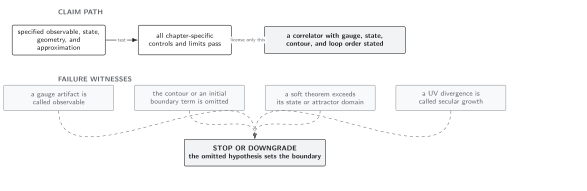
The crossing formula fails when slow variation, adiabatic state preparation, canonical matching, or attractor freeze-out fails; exact mode transport is then required. Schematic; not to scale.
References
Section titled “References”- Stewart, E. D., and D. H. Lyth, “A More Accurate Analytic Calculation of the Spectrum of Cosmological Perturbations Produced during Inflation,” Physics Letters B 302, 171–175 (1993), doi:10.1016/0370-2693(93)90222-S.
Original QFT.org content:CC BY 4.0, unless an item supplies different terms. Third-party material retains its own terms.