

Vacuum Polarization and Curved-Space Casimir Effects
Vacuum polarization is a local response of a specified state to geometry, topology, gauge background, or boundary data. Casimir observables are controlled differences or forces, not an absolute assignment of zero-point energy. The comparison must use the same local subtraction and finite bulk and surface couplings on both sides.
Required background. Renormalized Stress Tensor: Axioms and Curvature Ambiguities supplies the finite curvature freedom; Curved-Space Renormalization Schemes: Domains and Translation supplies scheme matching; Green Functions and Causal Propagators supplies the two-point kernels.
Helpful background. Local Covariance, Isometries, and Background Embeddings explains comparisons between backgrounds; Spectra, Resolvents, and Functional Calculus supplies the spectral representation.
Relative local observables
Section titled “Relative local observables”For two Hadamard states or boundary configurations whose local field operator agrees near , define
Their common Hadamard singularity cancels, so in a region where is smooth,
and
On this page the stress convention is
Because the same local finite curvature tensor is added to both terms, it cancels in a same-background state difference. It need not cancel when the geometries, boundary embeddings, or finite surface couplings differ. This is why a relative observable is stronger than an unqualified “renormalized vacuum energy.”
Boundary-induced singularities also deserve a separate qualification. At fixed positive proper distance from a smooth boundary, the relative two-point function is well defined under standard local boundary conditions. As the boundary is approached, additional surface singularities appear and require the boundary treatment developed later in this chapter. Deutsch and Candelas exhibit this near-surface stress behavior explicitly Deutsch and Candelas 1979, §§II–IV, pp. 3065–3074.
First application: an ultrastatic spectral difference
Section titled “First application: an ultrastatic spectral difference”Let
and let be positive and self-adjoint with boundary condition . Write
The ground-state equal-time kernel is formally
Choose two configurations with identical local geometry and matched high-frequency boundary data in the comparison region. After subtracting a common analytic high-mode expansion, compute
Here is the integrated local spectral asymptotic through the required order and restores its analytically summed remainder. The two spectra need not admit a meaningful term-by-term pairing; the subtraction is organized by a common spectral parameter or heat kernel.
For a one-parameter family such as a boundary separation , the relative vacuum energy is formally
and the force is
This derivative is insensitive to -independent bulk constants, but it can retain dependence on allowed -dependent surface or geometric counterterms. Heat-kernel coefficients identify precisely which local bulk and boundary pieces require matching Vassilevich 2003, §§2.2 and 5.2, pp. 288–294, 326–331.
Useful checks are the flat limit at fixed proper separation, the large-mass suppression of nonlocal polarization, symmetry under the isometries preserved by , stress conservation in the interior, and agreement between the stress discontinuity and after surface terms are included.
Adversarial absolute-energy test
Section titled “Adversarial absolute-energy test”Quote one finite value of and change the finite coefficients of or the conserved curvature tensors. The number changes while the state, field equation, and local singular subtraction remain the same. Calling that number an absolute observable overstates the calculation.
Now form a same-background state difference or a boundary force with identical finite couplings. The common bulk ambiguity cancels; only configuration-dependent local surface terms and the nonlocal response remain. The strongest claim is therefore the explicitly matched difference or force, with its domain away from unresolved boundary singularities—not an absolute local vacuum energy.
Polarization and failure maps
Section titled “Polarization and failure maps”The structure map shows the common local subtraction shared by both configurations and the later formation of a difference.

Scheme-independent content comes from a matched state, topology, or boundary comparison, while surface terms remain explicit; the map is schematic and not to scale.
The failure map asks whether a finite number survived a change of local curvature or surface prescription.
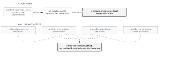
Relative stress, force, and topology dependence have different cancellation conditions and must be reported separately; the map is schematic and not to scale.
Use Domain and failure conditions. Record the background-identification map, state, boundary operator, proper distances, spectral measure, common subtraction, bulk and surface finite couplings, convergence, and the observable actually compared.
Mode-Sum and Numerical Renormalization develops the high-mode algorithm. Boundaries, Surface Counterterms, and Boundary Stress owns the surface limit. Chapter 13 owns cosmological-constant naturalness rather than this local comparison.
References
Section titled “References”- David Deutsch and Paul Candelas, “Boundary Effects in Quantum Field Theory,” Physical Review D 20 (1979), 3063–3080, DOI.
- Dmitri V. Vassilevich, “Heat Kernel Expansion: User’s Manual,” Physics Reports 388 (2003), 279–360, DOI, arXiv:hep-th/0306138.
Original QFT.org content:CC BY 4.0, unless an item supplies different terms. Third-party material retains its own terms.