Heat Kernels and the Schwinger–DeWitt Expansion

The Schwinger–DeWitt expansion is a short-proper-time asymptotic expansion of a heat kernel. It determines local ultraviolet divergences and, with a mass hierarchy, a local large-mass expansion. It does not by itself determine global spectra, late proper time, quantum state, absorptive parts, or causal response.

Required background. One-Loop Matter Effective Actions in Curved Space supplies the Hessian; Proper-Time, Zeta, and Determinant Prescriptions supplies the heat trace; and Asymptotic Scales, Remainders, Uniformity, and Optimal Truncation supplies the meaning of an asymptotic rather than convergent series.

Helpful background. Dimensional Regularization and Minimal Subtraction connects coefficients to poles, and Levi–Civita Connections, Geodesics, and Riemann Curvature fixes the geometric tensors.

The off-diagonal heat kernel

Let

$$\mathcal D=-\bigl(g_E^{\mu\nu}\nabla_\mu\nabla_\nu+\mathcal E\bigr)$$

act on a vector bundle over a smooth Riemannian manifold without boundary. Its heat kernel solves

$$(\partial_s+\mathcal D_x)K(s;x,x')=0, \qquad \lim_{s\downarrow0}K(s;x,x')=\delta(x,x')\mathbf1.$$

Inside a convex normal neighborhood the parametrix has the form

$$K(s;x,x')\sim \frac{\Delta^{1/2}(x,x')}{(4\pi s)^{d/2}} e^{-\sigma(x,x')/(2s)} \sum_{n=0}^\infty a_n(x,x')s^n,$$

where $\sigma$ is one-half the squared geodesic distance and $\Delta$ is the Van Vleck determinant. Substitution into the heat equation gives transport equations along the geodesic, beginning with $a_0(x,x')=\mathbf1$ after the displayed $\Delta^{1/2}$ has been factored. Coincidence limits $[a_n]=a_n(x,x)$ are local polynomials in $\mathcal E$, bundle curvature, Riemann curvature, and covariant derivatives. The general Laplace-type construction and its locality are reviewed in Vassilevich 2003, §§ 2.1 and 4.1.

Taking the trace gives

$$\operatorname{Tr}e^{-s\mathcal D} \sim\frac1{(4\pi s)^{d/2}} \sum_{n=0}^\infty s^n \int\mathrm d^dx\sqrt{g_E}\,\operatorname{tr}[a_n(x)].$$

Some literature labels these integrated terms $a_0,a_2,a_4,\ldots$ by mass dimension. This chapter labels the coefficient multiplying $s^n$ by $a_n$; thus its $a_2$ is Vassilevich’s $a_4$.

First application: poles through curvature squared

For the scalar operator

$$\mathcal L_E=\mathcal D+m^2, \qquad \mathcal E=\xi R_E,$$

the mass factor is exact:

$$\operatorname{Tr}e^{-s\mathcal L_E} =e^{-m^2s}\operatorname{Tr}e^{-s\mathcal D}.$$

In four dimensions, only the combinations $m^4a_0/2$, $-m^2a_1$, and $a_2$ multiply the ultraviolet pole. For a scalar bundle with vanishing connection curvature,

$$a_1=\left(\xi+\frac16\right)R_E,$$ $$\begin{aligned} a_2={}&\frac1{180}(R_{\mu\nu\rho\sigma}^2-R_{\mu\nu}^2) +\frac12\left(\xi+\frac16\right)^2R_E^2\\ &+\left(\frac1{30}+\frac\xi6\right)\nabla_E^2R_E. \end{aligned}$$

This follows directly from the universal coefficients Vassilevich 2003, Eqs. (4.26)–(4.28). The bundle case adds $\operatorname{tr}\Omega_{\mu\nu}\Omega^{\mu\nu}/12$. The coefficient dimensions give an immediate check: $[a_n]=2n$ in mass units.

The expansion also yields the local large-mass series after termwise proper-time integration,

$$\Gamma_E^{(1)}\sim -\frac12\frac1{(4\pi)^{d/2}} \sum_n m^{d-2n}\Gamma\!\left(n-\frac d2\right) \int\sqrt{g_E}\,\operatorname{tr}a_n,$$

with poles and logarithms treated by renormalization. Its control parameters are not merely “large $m$” but

$$\frac{|\mathcal R|}{m^2}\ll1, \qquad \frac{|\nabla^2\mathcal R|}{m^2|\mathcal R|}\ll1, \qquad \frac{p^2}{m^2}\ll1$$

for the curvatures and momenta retained.

Exact circle check and the large-s failure

For $-\partial_x^2+m^2$ on a circle of length $L$,

$$K(s)=\frac{L}{\sqrt{4\pi s}}e^{-m^2s} \left[1+2\sum_{q=1}^\infty e^{-q^2L^2/(4s)}\right].$$

At fixed $L$, every $q\ne0$ term is smaller than any power of $s$ as $s\downarrow0$. Therefore all local coefficients equal their line values, yet the exact determinant knows about $L$ through the winding terms. At large $s$, the lowest eigenvalue controls the trace and the local series is not an approximation. This is an explicit adversarial case: a perfect match of every power-series coefficient still fails to reconstruct the global infrared determinant.

The structure map places local heat-kernel asymptotics on only one branch of the determinant. Inspect the separate arrows to thresholds, nonlocal form factors, and imaginary parts.

The Schwinger–DeWitt series controls the local $s\downarrow0$ branch; topology, large-$s$ behavior, spectral cuts, and real-time response require additional data. Schematic; not to scale.

Domain and failure conditions

The displayed expansion assumes a smooth Laplace-type operator and a local convex neighborhood. Boundaries generate half-integer terms; cones may generate tip terms and logarithms; nonminimal operators require reduction; zero modes dominate large $s$; and Lorentzian state data are absent. See the canonical Domain and failure conditions.

The failure map’s local-expansion branch is decisive: extending a truncated $s\downarrow0$ series through $s\sim m^{-2}$ or into the infrared has no asymptotic warrant unless an independent uniform remainder estimate is supplied.

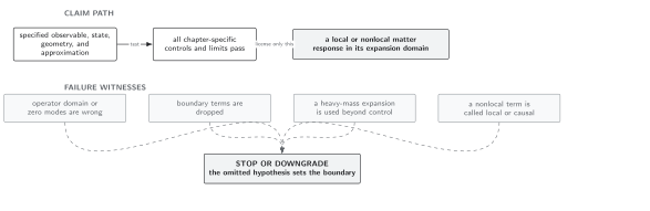
Small proper time and a controlled curvature or mass hierarchy license local coefficients; large proper time and global spectral sectors do not. Schematic; not to scale.

Handoffs

Seeley–DeWitt Coefficients and Curvature Invariants derives the transport recursion. Heat Kernels with Boundaries and Conical Singularities changes the domain and asymptotic structure. Matter-Induced Nonlocal Form Factors retains the momentum dependence that a finite local series discards.

References

• Avramidi, Ivan G. “Covariant Techniques for Computation of the Heat Kernel.” Reviews in Mathematical Physics 11 (1999): 947–980. DOI. Open PDF.
• Vassilevich, Dmitri V. “Heat Kernel Expansion: User’s Manual.” Physics Reports 388 (2003): 279–360. DOI. Open PDF.