Particles, Detectors, and Nonadiabatic Production

“Particle production” can name several inequivalent observations: occupation of an out-mode basis, excitation of a localized detector, a KMS detailed-balance relation, or transported stress-energy. These notions agree only under additional stationarity, asymptotic, switching, localization, and energy-accounting assumptions. This chapter makes those assumptions explicit and treats disagreement as physical information rather than a notational nuisance.

The recurring scalar convention is

$$P_\xi=\Box_g+m^2+\xi R, \qquad \xi_{\mathrm{conf}}=-\frac16$$

in four dimensions. The causal propagator is $E=G_{\mathrm{ret}}-G_{\mathrm{adv}}$, so $[\Phi(f),\Phi(h)]=-iE(f,h)\mathbf1$. A detector response instead uses a state-dependent Wightman function. Neither the commutator nor a detector click by itself defines an invariant particle density.

Helpful background. Vacuum Ambiguity, Time Flow, and Observer Dependence explains why positive frequency is additional data; Green Operators, Causal Propagators, and State-Dependent Two-Point Functions separates response from state covariance; Localized Probe and Detector Models and Particle Detectors versus Field Observables supply the operational framework.

Choose the observable before calculating

Four questions determine the route.

1. Is there a stationary or asymptotically stationary time flow? If yes, positive frequency and in/out number operators may be meaningful.
2. Is the measurement localized along a worldline or worldtube? If yes, specify detector gap, coupling, trajectory, switching, and smearing.
3. Is thermality claimed? Test KMS analyticity or long-time detailed balance with respect to a normalized time generator.
4. Is energy transported? Compute a renormalized stress flux and identify the work done by a time-dependent metric, electric field, or boundary.

Fulling’s nonuniqueness result shows why a generic curved spacetime does not supply one canonical particle basis Fulling 1973, pp. 2850–2862. Parker’s expanding-universe calculation and Unruh’s accelerated-detector calculation are controlled precisely because they add different operational structures Parker 1968, pp. 562–564, Unruh 1976, pp. 870–892.

The construction map displays the common sequence. Inspect the two checkpoints: an asymptotic limit and energy balance are needed before a computed transition becomes a qualified particle statement.

Mode number, detector response, Stokes production, and flux follow different controlled paths through the same operational construction; the map is schematic and not to scale.

Chapter guide

1. Particles, Local Observables, and Detector Dependence separates number, clicks, correlators, and stress flux.
2. Mode Bases, In/Out States, and Number Operators states when asymptotic particle counting is controlled.
3. Detector Response Along Curved and Accelerated Worldlines derives the response from the pulled-back two-point function.
4. Switching, Smearing, Finite-Time Response, and Transients controls finite duration and ultraviolet sensitivity.
5. Particle Creation in Time-Dependent Backgrounds computes in/out Bogoliubov production and its energy.
6. Adiabaticity, Stokes Phenomena, and Production Rates treats complex turning points, interference, and error domains.
7. Parametric-Oscillator and Solvable Production Benchmarks supplies exact quench fixtures.
8. Unruh Effect and Uniformly Accelerated Detectors derives acceleration-temperature detailed balance.
9. Tolman Redshift, KMS Structure, and Local Temperature distinguishes global KMS data from calibrated local temperature.
10. Acceleration, Gravity, and the Limits of Equivalence-Principle Arguments isolates local kinematics from curvature, state, and horizon data.
11. Moving Mirrors and the Dynamical Casimir Effect compares Bogoliubov particles, boundary work, and outgoing flux.
12. Schwinger and Gravitational Production: A Controlled Comparison identifies shared turning-point mathematics and different physics.

Domain and failure conditions

This table is the chapter’s canonical comparison. Each row licenses only the stated observable; no row is an automatic substitute for another.

Construction	State, geometry, and trajectory	Basis or interaction	Switching, asymptotics, and regulator	Reported observable	Energy accounting	Licensed claim and decisive failure
In/out number	In-state; asymptotically stationary past and future	Complete normalized in/out bases	Wavepackets or volume normalization; controlled asymptotic regions	$\langle N_f^{\mathrm{out}}\rangle$	Out energy from $\omega_fN_f$ plus vacuum and interference terms as applicable	Asymptotic occupation; fails without an out splitting
Instantaneous basis	State on one slice; chosen canonical variables	Time-local diagonalization or WKB basis	Adiabatic order and phase convention	$n_{\mathbf k}(t)$	Basis Hamiltonian, not automatically local stress energy	Diagnostic occupation; fails as an invariant under time-dependent basis changes
Localized detector	Hadamard state; declared worldline	Probe gap and field coupling	Smooth switching, spatial profile, perturbative order	Excitation probability or transition rate	Work supplied by detector control and trajectory	Response of that apparatus; fails as pre-existing density when protocol changes it
KMS or detailed balance	Stationary state and normalized flow	Stationary detector or algebra automorphism	Long-time or exact KMS domain	Spectral ratio $e^{-\beta\Omega}$	Equilibrium exchange with respect to the same generator	Thermality for that flow; fails for finite transients or a rescaled generator
Stress flux	Renormalizable state; local geometry	Local $T_{\mu\nu}$ and observer or null direction	Locally covariant subtraction and boundary data	$\langle T_{\mu\nu}\rangle_{\mathrm{ren}}u^\mu n^\nu$	Direct transported energy with source or boundary work	Local flux; fails if subtraction or conservation is uncontrolled
WKB or Stokes production	Specified in-state and analytic frequency profile	Complex turning points and connection matrices	Saddle set, Stokes graph, prefactor, uniform error	Semiclassical $\lvert\beta_{\mathbf k}\rvert^2$	Compare integrated energy with background work	Asymptotic production estimate; fails outside its saddle and asymptotic regime

The failure map turns the last column into an explicit stop rule. Inspect which omitted hypothesis—basis invariance, switching, curvature, or asymptotic duration—causes the proposed claim to be narrowed.

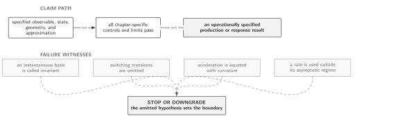
An omitted operational hypothesis sets the boundary of the particle claim; the validity and failure map is schematic and not to scale.

A reusable operational contract

Before reporting a number, name:

• the field state and its ultraviolet class;
• the spacetime, boundary condition, and observer or detector trajectory;
• the mode basis or detector interaction and gap;
• switching, smearing, regulator, and order of limits;
• the observable—number, probability, rate, detailed-balance ratio, or flux;
• the asymptotic and approximation domain;
• the source of the measured energy and the first uncontrolled term.

For a smooth-switching Unruh–DeWitt detector, the leading response is

$$\mathcal F_\chi(\Omega) = \int\mathrm d\tau\,\mathrm d\tau'\, \chi(\tau)\chi(\tau') e^{-i\Omega(\tau-\tau')} W_\omega(x(\tau),x(\tau')).$$

Changing $\chi$ or $x(\tau)$ can change $\mathcal F_\chi$ while the field state remains fixed. Louko and Satz show how smooth switching and the Hadamard property give a regulator-free curved-spacetime response formula Louko and Satz 2008, §§2–4. That result is operationally sharp, but it is not a theorem that $\mathcal F_\chi$ equals a local particle density.

Abstract detector instruments remain in Volume XIII. Communication protocols begin in Chapter 5, local stress-tensor renormalization in Chapter 7, collapse-induced Hawking radiation in Chapter 6, and cosmological applications in Chapter 14.

References

• S. A. Fulling, “Nonuniqueness of Canonical Field Quantization in Riemannian Space-Time,” Physical Review D 7 (1973), 2850–2862, DOI.
• Jorma Louko and Alejandro Satz, “Transition Rate of the Unruh–DeWitt Detector in Curved Spacetime,” Classical and Quantum Gravity 25 (2008), 055012, DOI, arXiv:0710.5671.
• Leonard Parker, “Particle Creation in Expanding Universes,” Physical Review Letters 21 (1968), 562–564, DOI.
• William G. Unruh, “Notes on Black-Hole Evaporation,” Physical Review D 14 (1976), 870–892, DOI.