

Renormalized Currents and Charge Density
A renormalized charge current is a local, gauge-covariant composite operator; a charge density is its projection onto a specified observer. Point splitting must transport both gauge and spacetime indices before coincidence, and the result is accepted only after its Ward identity, finite charge normalization, state, and boundary flux have been checked.
Required background. Wick Polynomials and Hadamard Point Splitting supplies the subtraction; Gauge Fields, Gauge Fixing, and Ghosts on Curved Backgrounds supplies gauge-covariant propagation; Coupling to Background Gauge Fields and Bundles supplies the background Ward identity.
Helpful background. Contact Terms and Renormalized Operator Products controls inserted divergences; Regulated Jacobians and Measure Variation distinguishes an anomalous current.
Gauge-covariant current splitting
Section titled “Gauge-covariant current splitting”For a complex scalar of charge ,
With the current convention
the classical scalar current is
Let . It transforms at both endpoints. Along the unique geodesic in a convex normal neighborhood, let
be the gauge parallel transporter, and let transport a tangent index. A gauge-covariant point-split definition is schematically
The charged Hadamard parametrix obeys the same endpoint transformation law as . The star on the primed derivative denotes the conjugate representation. Detailed Hadamard recursions for the charged scalar and the required current limit are given by Balakumar and Winstanley 2020, §§3–4, pp. 13–27 of the Open PDF.
In an anomaly-free theory the allowed finite current shift in four dimensions includes
which is the response to a finite term. It is identically conserved and changes the background gauge-coupling prescription. It is neither state dependence nor an anomaly.
The proper-time point-splitting calculation displays both the charged-current divergence structure and the electromagnetic terms induced in the stress counterterms Herman and Hiscock 1996, §§II–IV, pp. 3287–3293.
First application: stationary charged scalar
Section titled “First application: stationary charged scalar”Assume a stationary globally hyperbolic region with Killing field , a gauge field stationary up to a gauge transformation, a stationary Hadamard state, and boundary conditions with declared flux. Evaluate the split expression in a symmetry-adapted frame. The checks are
where the second sign follows from the functional variations displayed above. In a static spherical chart, stationarity and angular symmetry reduce the first identity to
Thus is the conserved radial flux between sources or boundaries. It need not vanish in a nonequilibrium stationary state.
For a unit future-directed observer , the measured charge density is
If is boosted along a unit spatial vector , then
The current is geometric; “the density” is not observer independent. Report , the frame normalization, the state, and the finite prescription with every density value. Concrete charged-black-hole calculations use precisely this combination of Hadamard subtraction and flux checks Klein and Zahn 2021, §§II–IV, pp. 2–8.
Adversarial test: omit the transporter
Section titled “Adversarial test: omit the transporter”Under ,
The derivative at coincidence therefore differentiates the endpoint phase. If one subtracts untransported coordinate components, the apparent finite current acquires terms proportional to derivatives of or depends on the chosen splitting path. The factor cancels that phase; changing the path then probes the enclosed field strength and must be controlled in the coincidence expansion.
The strongest result without parallel transport is a gauge-fixed regulator diagnostic. It is not a local current and cannot enter a Ward identity or an observer-independent charge balance.
Current and failure maps
Section titled “Current and failure maps”The structure map emphasizes that endpoint transport is part of the observable definition, not a cosmetic step after subtraction.

Gauge and tangent transport precede coincidence, while observer projection follows construction of the geometric current; the map is schematic and not to scale.
The failure map separates gauge-phase contamination, a physical boundary flux, a finite charge prescription, and a genuine anomaly.
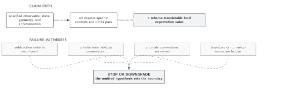
A finite component is not yet a covariant conserved current; the map is schematic and not to scale.
Use Domain and failure conditions. Check the charged field equation in both arguments, endpoint gauge law, tangent transport, coincidence order, divergence, stress-force sign, boundary flux, observer normalization, dimensions, and finite prescription.
Check your understanding
Section titled “Check your understanding”Why is for a smooth Abelian field strength?
Solution
Antisymmetry gives . The commutator contracts the symmetric Ricci tensor with the antisymmetric , so the result vanishes.
Vacuum Polarization and Curved-Space Casimir Effects treats scheme-controlled differences; Spin, Gauge, and Gravitational-Anomaly Responses treats anomalous Ward identities. Transport and hydrodynamic constitutive currents belong to Volume XI.
References
Section titled “References”- Visakan Balakumar and Elizabeth Winstanley, “Hadamard Renormalization for a Charged Scalar Field,” Classical and Quantum Gravity 37 (2020), 065004, DOI, Open PDF.
- Rhett Herman and William A. Hiscock, “Renormalization of the Charged Scalar Field in Curved Space,” Physical Review D 53 (1996), 3285–3295, DOI, arXiv:gr-qc/9509015.
- Christiane Klein and Jochen Zahn, “The Renormalized Charged Scalar Current in the Reissner–Nordström–de Sitter Spacetime,” Physical Review D 104 (2021), 025009, DOI, arXiv:2104.06005.
Original QFT.org content:CC BY 4.0, unless an item supplies different terms. Third-party material retains its own terms.