Long-Distance Quantum Corrections

Long-distance quantum-gravity predictions come from nonanalytic low-momentum terms. A local counterterm produces a momentum polynomial and therefore only contact terms or source-size structure; it cannot change a massless logarithm or square-root branch cut. Fourier transformation turns those nonanalyticities into power-law tails, but the coefficient of a coordinate-space “potential” remains sensitive to field variables, coordinates, and Born-iteration conventions.

Required background. One-Loop Graviton EFT supplies the on-shell nonanalytic amplitude; Graviton and Matter Nonlocal Form Factors supplies its curvature representation; and Modes, Virtualities, and EFT Scale Separation separates potential, radiation, and hard regions.

Helpful background. Hilbert Positivity and Unitary Evolution supplies the cut interpretation, while Matching Conditions Beyond Tree Level supplies subtraction of iterated lower-order exchange.

Nonanalyticity becomes a spatial tail

With the site spatial Fourier convention and $r=\lvert\boldsymbol r\rvert>0$,

$$\begin{aligned} \int\frac{\mathrm d^3\boldsymbol q}{(2\pi)^3}\, \frac{e^{i\boldsymbol q\cdot\boldsymbol r}}{\boldsymbol q^2} &=\frac1{4\pi r},\\ \int\frac{\mathrm d^3\boldsymbol q}{(2\pi)^3}\, \frac{e^{i\boldsymbol q\cdot\boldsymbol r}}{\lvert\boldsymbol q\rvert} &=\frac1{2\pi^2r^2},\\ \int\frac{\mathrm d^3\boldsymbol q}{(2\pi)^3}\, e^{i\boldsymbol q\cdot\boldsymbol r} \log\!\left(\frac{\boldsymbol q^2}{\mu^2}\right) &=-\frac1{2\pi r^3}. \end{aligned}$$

The last two equalities are distributional; the displayed forms omit contact terms supported at $\boldsymbol r=0$. Changing $\mu$ adds a constant in momentum space and therefore changes only such a contact term. This is why the $r>0$ tail is independent of the subtraction scale.

A convenient derivation starts from

$$I_\alpha(r) =\int\frac{\mathrm d^3\boldsymbol q}{(2\pi)^3} e^{i\boldsymbol q\cdot\boldsymbol r} (\boldsymbol q^2)^{-\alpha} =\frac{\Gamma(\frac32-\alpha)} {4^\alpha\pi^{3/2}\Gamma(\alpha)} (r^2)^{\alpha-\frac32}.$$

The second identity follows at $\alpha=1/2$. Differentiating $-\partial_\alpha I_\alpha$ at $\alpha=0$ gives the logarithm for $r>0$; the pole at $\alpha=0$ encodes the omitted local distribution.

The structure map carries precisely these nonanalytic terms, rather than an arbitrary off-shell potential, into the long-distance observable.

For noncoincident points, $1/\boldsymbol q^2$, $1/\lvert\boldsymbol q\rvert$, and $\log\boldsymbol q^2$ generate $1/r$, $1/r^2$, and $1/r^3$ behavior; analytic momentum terms contribute only local or finite-size data. The map is schematic and not to scale.

First application: two heavy sources

For nonrelativistic scattering of masses $m_1$ and $m_2$, organize the low-momentum amplitude after subtracting the appropriate iteration of lower-order exchange as

$$\mathcal M(\boldsymbol q) =\mathcal M_{\mathrm N}(\boldsymbol q) \left[ 1+a_{\mathrm{cl}}G(m_1+m_2) \lvert\boldsymbol q\rvert +a_{\mathrm q}G\boldsymbol q^2 \log\!\left(\frac{\boldsymbol q^2}{\mu^2}\right) +\cdots \right],$$

where $\mathcal M_{\mathrm N}\propto Gm_1m_2/\boldsymbol q^2$. The coefficients $a_{\mathrm{cl}}$ and $a_{\mathrm q}$ depend on the normalization and on which complete set of diagrams defines the amplitude; no universal numerical value is asserted here.

The square-root contribution transforms as $1/\lvert\boldsymbol q\rvert$ and gives an absolute $1/r^2$ correction. Although it can arise from loop integrals, it is classical: relative to the Newtonian result it scales as

$$\delta_{\mathrm{cl}} \sim\frac{G(m_1+m_2)}{r}.$$

The logarithm transforms as $1/r^3$ and gives

$$\delta_{\mathrm q} \sim\frac{G}{r^2} =\frac{\ell_{\mathrm{Pl}}^2}{r^2}$$

up to the reduced-Planck normalization and a process-dependent coefficient. Restoring units places an explicit $\hbar$ in the quantum term but not in $\delta_{\mathrm{cl}}$. The separation of classical and quantum nonanalytic pieces, including the alternative Born-subtracted potential, is worked out in Bjerrum-Bohr, Donoghue, and Holstein 2003, §§2.1–4.1.

A chosen nonrelativistic convention may package the result as

$$V(r) =-\frac{Gm_1m_2}{r} \left[ 1+\widetilde a_{\mathrm{cl}} \frac{G(m_1+m_2)}r +\widetilde a_{\mathrm q}\frac{G}{r^2} +\cdots \right].$$

This formula is useful only together with its coordinate choice, field definition, source normalization, and subtraction of iterated exchange. A local field redefinition or coordinate transformation can move terms between $V$, momentum-dependent operators, and contact interactions. The invariant on-shell amplitude—and derived quantities such as a scattering angle or a relational time delay—does not move when the whole dictionary is transformed. Donoghue’s original EFT calculation emphasizes that the long-range prediction is tied to nonanalytic low-energy propagation Donoghue 1994, §§III–V, pp. 3878–3886.

Classical post-Newtonian comparison

Both the first post-Newtonian term and the leading quantum tail may be generated in a one-loop representation, but their expansion parameters differ:

$$\frac{\delta_{\mathrm q}}{\delta_{\mathrm{cl}}} \sim\frac1{(m_1+m_2)r}.$$

For macroscopic sources at a common separation the quantum term is far smaller. This comparison assumes a point-particle description valid at $r$; finite-size tidal operators can introduce additional powers of the source radius. It also assumes the same conservative observable, since radiation-reaction and dissipative tails use different boundary conditions.

Adversarial short-distance extrapolation

The tail calculation requires

$$r\gg \max\!\left( \Lambda_{\mathrm{EFT}}^{-1}, \ell_{\mathrm{Pl}}, G(m_1+m_2), R_{\mathrm{source}} \right)$$

for a weak-field point-source application. Driving $r$ to $\ell_{\mathrm{Pl}}$ makes $G/r^2$ order unity, so every higher loop and higher-derivative operator can compete. The small long-distance coefficient contains no controlled information about the resulting ultraviolet theory. If $G(m_1+m_2)/r$ fails first, the problem is instead a classical strong-field breakdown.

Domain and failure conditions

The chapter comparison table requires the amplitude normalization, light spectrum, momentum region, subtraction of iterations, source model, coordinate or relational observable, and cutoff. The Fourier identities license tails only for $r>0$; contact terms and finite-size data must be matched separately.

The failure map stops the calculation before a long-distance series is extrapolated through its own breakdown scale.

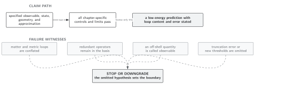
Long-distance nonanalytic tails are robust only where quantum, post-Newtonian, finite-size, and derivative expansions are simultaneously small; their growth marks loss of control, not a selected UV completion. The map is schematic and not to scale.

References

• Bjerrum-Bohr, N. E. J., J. F. Donoghue, and B. R. Holstein. “Quantum Gravitational Corrections to the Nonrelativistic Scattering Potential of Two Masses.” Physical Review D 67, 084033 (2003). doi:10.1103/PhysRevD.67.084033. Open PDF
• Donoghue, J. F. “General Relativity as an Effective Field Theory: The Leading Quantum Corrections.” Physical Review D 50, 3874–3888 (1994). doi:10.1103/PhysRevD.50.3874. Open PDF