Baryogenesis Inputs and the Cosmological Yield

A cosmological baryogenesis handoff propagates a supplied CP-violating source and supplied charge-violation and washout rates through an accepted transition history. It does not infer CP violation from bubble nucleation, nor does it turn latent heat into a baryon source. Its output is a final yield with source, transport, washout, reheating, and entropy uncertainties kept distinct and correlated.

Required background. Expansion history, percolation, and completion supplies the accepted wall and reheating history. Anomalous charge violation and cosmology supplies the microscopic source, conversion, and washout interfaces.

Helpful background. Thermal nucleation supplies rate covariance, and thermal percolation and reheating supplies the plasma-history context.

Comoving charge transport

For a homogeneous coarse-grained baryon density $n_B$, write

$$\dot n_B+3Hn_B=S_B(t)-\Gamma_w(t)n_B.$$

Here $S_B$ is the net physical-volume source after the microscopic diffusion and anomalous-charge conversion problem has been solved, while $\Gamma_w$ is an effective washout rate with units of inverse time. Defining the comoving charge $N_B=a^3n_B$ gives

$$\dot N_B=a^3S_B-\Gamma_wN_B .$$

The exact linear solution is

$$\begin{aligned} N_B(t)={}&N_B(t_i) \exp\!\left[-\int_{t_i}^{t}\Gamma_w(u)\,du\right]\\ &+\int_{t_i}^{t}dt'\,a(t')^3S_B(t') \exp\!\left[-\int_{t'}^{t}\Gamma_w(u)\,du\right]. \end{aligned}$$

This integrating-factor expression is the central cosmological calculation. It makes the time ordering explicit: early charge is more strongly washed out, and a source after washout freezes out survives more efficiently.

The source input must declare the charge basis, sign convention, CP phases, wall orientation, wall profile and velocity, diffusion constants, thermal masses, damping rates, and conversion matrix. The washout input must declare whether it acts in the symmetric phase, broken phase, or both. Electroweak baryogenesis calculations require all of these ingredients; the Sakharov conditions alone do not determine their magnitude (Morrissey and Ramsey-Musolf 2012, §§ 3–5).

Entropy and the observable yield

The reported late-time quantity is normally

$$Y_B(t)=\frac{n_B(t)}{s(t)} =\frac{N_B(t)}{S_c(t)}, \qquad S_c(t)=a(t)^3s(t).$$

If reheating produces entropy,

$$\dot S_c=a^3\Sigma_s\geq0,$$

then

$$\dot Y_B =\frac{S_B}{s} -\Gamma_wY_B -Y_B\frac{\dot S_c}{S_c}.$$

The last term is dilution. If charge production and washout have ended before a later entropy injection,

$$Y_B^{\mathrm{after}} =\frac{Y_B^{\mathrm{before}}}{\Delta}, \qquad \Delta= \frac{S_c^{\mathrm{after}}}{S_c^{\mathrm{before}}}.$$

Using $n_B$ at one time and $s$ at another without this factor is not a harmless normalization choice. During reheating, temperature may be nonmonotonic, so an integration in $T$ must be split into monotonic branches. Time or e-fold number is safer.

Nonperturbative anomalous rates can be a leading uncertainty rather than a detail. D’Onofrio, Rummukainen, and Tranberg compute the Standard Model sphaleron rate across the electroweak crossover and exhibit its strong temperature dependence (D’Onofrio, Rummukainen, and Tranberg 2014, Eqs. (2)–(5) and Fig. 2). A beyond-Standard-Model transition requires its own controlled rate or an explicitly qualified approximation.

Supplied-input application

Given a joint sample

$$\mathcal D= \{a(t),T(t),S_c(t),v_w(t), S_B(t),\Gamma_w(t),C_{\mathcal D}\},$$

perform the following calculation:

1. verify that the history completed and that the source’s wall regime matches $v_w(t)$;
2. interpolate positive rates in logarithmic variables and signed sources with a method that preserves integrated charge;
3. integrate $N_B$ in time while monitoring the exact integrating-factor solution;
4. divide by the final $S_c$, after all declared entropy production;
5. repeat over joint samples from the full covariance $C_{\mathcal D}$.

Report the sign convention and the probability distribution of $Y_B$, not only a central magnitude. Correlations matter: the same wall velocity can enhance a microscopic source while shortening diffusion time, and the same reheating history can alter both washout and dilution.

Time-variable and normalization adversarial test

Compute the same history in cosmic time and in e-fold number $N=\log a$. Since $d/dt=H\,d/dN$, the second form is

$$\frac{dN_B}{dN} =\frac{a^3S_B}{H} -\frac{\Gamma_w}{H}N_B .$$

The final $N_B$ and $Y_B$ must agree within numerical tolerance. Then rescale the arbitrary comoving coordinate volume by a constant $c$: both $N_B$ and $S_c$ scale by $c$, while $Y_B$ remains unchanged. A code that changes the yield under either test has mixed physical and comoving densities or omitted a Jacobian.

Finally, insert a controlled entropy pulse after the source shuts off and verify $Y_B\mapsto Y_B/\Delta$. Failure of that check rejects the cosmological yield even if the microscopic source is sophisticated.

The structure map identifies where baryogenesis enters. Inspect how CP source and washout data attach to an already accepted wall history, followed by entropy normalization.

From microscopic charge inputs to the cosmological baryon yield. The diagram is schematic and not to scale; nucleation and latent heat do not replace a CP source, transport calculation, or washout rate.

The failure map makes the missing-input tests explicit. Inspect the separate stops for absent CP violation, omitted washout, inconsistent wall data, and untracked entropy production.

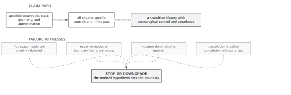
Failure conditions for the baryogenesis handoff. The diagram is schematic and not to scale; the final yield is licensed only after source, washout, expansion, and entropy histories are propagated together.

These restrictions refine the chapter’s domain and failure conditions.

Exercise

Let $a^3S_B=J_0$ and $\Gamma_w=\gamma$ be constant for $0<t<\tau$, with $N_B(0)=0$, and let both vanish afterward. A later reheating event increases $S_c$ by $\Delta$. Find the final yield.

Solution

During production,

$$N_B(\tau)= \int_0^\tau dt'\,J_0e^{-\gamma(\tau-t')} =\frac{J_0}{\gamma}(1-e^{-\gamma\tau}),$$

with the smooth limit $N_B=J_0\tau$ as $\gamma\to0$. If $S_{c,0}$ is the comoving entropy just before reheating, then

$$Y_B^{\mathrm{final}} =\frac{J_0(1-e^{-\gamma\tau})} {\gamma\,\Delta S_{c,0}}.$$

The exponential is washout; the factor $1/\Delta$ is later entropy dilution.

References

• D’Onofrio, M., K. Rummukainen, and A. Tranberg. “Sphaleron Rate in the Minimal Standard Model.” Physical Review Letters 113 (2014): 141602. DOI. Open PDF.
• Morrissey, D. E., and M. J. Ramsey-Musolf. “Electroweak Baryogenesis.” New Journal of Physics 14 (2012): 125003. DOI. Open PDF.