Conformal Transformations and Frame Changes

A Weyl rescaling can transport a classically conformal field theory between conformally related backgrounds, including its causal Green functions and suitably transported states. The map fails for masses and nonconformal curvature couplings, and renormalized composite operators can acquire local curvature terms and anomalies even when the classical equation is conformally covariant. A general “frame change” is therefore an equivalence only after fields, sources, units, state, boundary data, and renormalization prescriptions have all been transformed.

Required background. Covariant Scalar Fields and Curvature Coupling fixes the operator and signs; Local Covariance, Isometries, and Background Embeddings supplies the algebraic comparison.

Helpful background. Weyl Anomalies and Conformal Perturbation Theory supplies the quantum obstruction; Levi–Civita Connection, Geodesics, and Riemann Curvature supplies the curvature transformation.

The conformal wave operator

Let

$$\widetilde g_{\mu\nu} = \Omega^2g_{\mu\nu}, \qquad \Omega>0,$$

and set

$$c_d=\frac{d-2}{4(d-1)}.$$

With the site’s curvature convention, the massless conformal operator is

$$L_g = \Box_g-c_dR_g.$$

It obeys

$$L_{\widetilde g} \left( \Omega^{-(d-2)/2}\phi \right) = \Omega^{-(d+2)/2}L_g\phi.$$

Thus

$$\widetilde\phi = \Omega^{-(d-2)/2}\phi$$

maps solutions to solutions. In the chapter’s parameterization $P_\xi=\Box_g+m^2+\xi R$, this is

$$m=0, \qquad \xi=\xi_{\mathrm{conf}}=-c_d.$$

In four dimensions $\xi_{\mathrm{conf}}=-1/6$. Sources using $P=\Box+m^2-\zeta R$ instead quote $\zeta_{\mathrm{conf}}=+1/6$; these are the same operator.

The Green kernels transform as bidistributions:

$$G_{\widetilde g,\mathrm{ret/adv}}(x,y) = \Omega(x)^{-(d-2)/2} \Omega(y)^{-(d-2)/2} G_{g,\mathrm{ret/adv}}(x,y),$$

provided the conformal map preserves the relevant causal domain and boundary problem. The same law holds for $E$. A conformally transported state has

$$W_{\widetilde\omega}(x,y) = \Omega(x)^{-(d-2)/2} \Omega(y)^{-(d-2)/2} W_\omega(x,y).$$

This transports one state; it does not prove that the transported state is preferred by every observer or global completion.

The operator, Green-kernel, and two-point weights follow from the conformal scalar construction in Birrell and Davies 1982, §§3.2 and 6.2.

First application: Minkowski space and flat FLRW

In conformal time, a spatially flat FLRW metric is

$$\widetilde g_{\mu\nu} = a(\eta)^2\eta_{\mu\nu}.$$

For a massless conformally coupled scalar in $d$ dimensions, define

$$\chi = a^{(d-2)/2}\widetilde\phi.$$

Then

$$\left( \partial_\eta^2-\nabla^2 \right)\chi=0.$$

Transporting the Minkowski vacuum gives

$$W_{\mathrm{conf}}(x,y) = a(\eta_x)^{-(d-2)/2} a(\eta_y)^{-(d-2)/2} W_{\mathrm{Mink}}(x,y).$$

The FLRW Klein–Gordon normalization is preserved because the field weights cancel the scale factors from the unit normal and surface measure. This provides a useful round-trip check:

$$\widetilde\phi \xrightarrow{\ a^{(d-2)/2}\ } \chi \xrightarrow{\ a^{-(d-2)/2}\ } \widetilde\phi.$$

No gravitational particle production occurs relative to the conformally transported mode split for this exact massless conformal system. Detector response can still depend on the detector trajectory, switching, and conformal scaling of its coupling; the statement is not “all observables equal their Minkowski values.”

Where the equivalence fails

Now keep the same FLRW geometry but take $m\ne0$ or $\xi\ne\xi_{\mathrm{conf}}$. The rescaled mode equation contains

$$a^2m^2 +a^2(\xi-\xi_{\mathrm{conf}})R.$$

The Minkowski equation is not recovered. This adversarial test distinguishes a genuine conformal transport from a change of variables that merely relocates the time dependence.

Renormalized composites add a second obstruction. Products such as $\phi^2(x)$ and $T_{\mu\nu}(x)$ require a local subtraction scale. Under Weyl rescaling, the subtraction and local curvature counterterms transform, and in even dimensions the trace can contain a state-independent local anomaly:

$$\langle T^\mu{}_\mu\rangle_{\mathrm{ren}} \ne0$$

even for a classically conformal theory. Its coefficients and removable total-derivative terms depend on the field content and renormalization convention. Chapter 7 treats that classification; the present page claims only the classical and two-point transport law before composite renormalization.

Wald’s axiomatic analysis shows why a conformally invariant classical equation can nevertheless acquire a local quantum trace term Wald 1978, pp. 1477–1484; the modern locally covariant setting and renormalization freedom are reviewed in Hollands and Wald 2015, §§3–4.

A scalar–tensor “Jordan-to-Einstein frame” transformation is broader still. To compare predictions, one must transform the metric, dynamical scalar, matter fields, sources, rods and clocks, boundary conditions, functional measure, and renormalized couplings. Comparing the same numerical coordinate interval or holding one frame’s detector action fixed is not a frame-invariant experiment.

Construction and failure maps

The construction map shows what a valid conformal transport must carry: the operator and causal domain, the conserved solution space, and the local algebra. The state is transported only after these layers agree.

Classical conformal covariance reaches the state layer only after the operator, causal domain, and algebra have been transported consistently; the map is schematic and not to scale.

In the failure map, an observable-assignment change detects omitted field weights, boundary data, or renormalized curvature terms. A mass or wrong curvature coupling fails earlier, at the operator box.

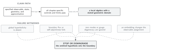
Exact transport is licensed for the declared conformal field and causal-boundary problem; masses, nonconformal couplings, and anomalies set explicit boundaries. Schematic and not to scale.

See Domain and failure conditions for the chapter comparison. On this page the decisive checks are the conformal operator identity, the Green-kernel weight, preservation of the Klein–Gordon normalization, transformation of the state and detector, and inclusion of anomaly terms for renormalized composites.

Check your understanding

Why do both arguments of a conformally transported two-point function carry the field weight?

Solution

Each field insertion transforms as $\widetilde\phi(x)=\Omega(x)^{-(d-2)/2}\phi(x)$. Therefore the expectation value of two insertions receives one factor at $x$ and one at $y$. The same weights also make the transformed causal kernel invert $L_{\widetilde g}$ against the transformed volume delta distribution.

Weyl anomalies belong to Volume IX and Local Observables, Stress Tensors, and Anomalies. Full quantum equivalence of scalar–tensor frames requires a separate gravity-sector analysis.

References

• N. D. Birrell and P. C. W. Davies, Quantum Fields in Curved Space, Cambridge University Press (1982), DOI, §§3.2 and 6.2.
• Stefan Hollands and Robert M. Wald, “Quantum Fields in Curved Spacetime,” Physics Reports 574 (2015), 1–35, DOI, Open PDF, §§2–4.
• Robert M. Wald, “Trace Anomaly of a Conformally Invariant Quantum Field in Curved Spacetime,” Physical Review D 17 (1978), 1477–1484, DOI.