Cubic Interactions and Bispectrum Shapes

The inflationary bispectrum is the first correlator sensitive to interactions. A momentum-space “shape” is not itself a model: its normalization and limiting behavior also depend on the constraint solution, nonlinear field definition, initial state, contour, and treatment of bulk and boundary terms.

Required background. In-in cosmological correlators supplies the real-time expectation value; contours and initial boundaries supplies state and endpoint terms; the EFT of inflation supplies the operator expansion; and Mukhanov–Sasaki modes supplies normalized external legs.

Helpful background. Power spectra and freeze-out fixes two-point normalization, while local field redefinitions clarifies equation-of-motion operators.

From a cubic operator to a momentum shape

Define the dimensionful power spectrum and bispectrum by

$$\begin{aligned} \langle\zeta_{\mathbf k}\zeta_{\mathbf k'}\rangle &=(2\pi)^3\delta^3(\mathbf k+\mathbf k')P_\zeta(k),\\ \langle\zeta_{\mathbf k_1}\zeta_{\mathbf k_2}\zeta_{\mathbf k_3}\rangle &=(2\pi)^3\delta^3(\mathbf k_1+\mathbf k_2+\mathbf k_3) B_\zeta(k_1,k_2,k_3). \end{aligned}$$

For example, the local convention is

$$B_\zeta^{\rm local}= \frac65f_{\rm NL}^{\rm local} \left[P_\zeta(k_1)P_\zeta(k_2)+2\ \text{permutations}\right].$$

Derivative interactions in a single-clock EFT instead tend to peak for comparable momenta. In the Goldstone limit, reduced sound speed generates operators schematically proportional to

$$(1-c_s^{-2})\dot\pi\frac{(\partial_i\pi)^2}{a^2}, \qquad (1-c_s^{-2})\dot\pi^3,$$

with independent Wilson-coefficient combinations in the most general EFT. Their in-in time integrals contain the total energy $K=k_1+k_2+k_3$ and produce equilateral or orthogonal combinations depending on the relative coefficient. The general single-field calculation and shape classification are developed in Chen et al. 2007, §§3–5, Eqs. (3.1)–(5.10).

The first application is to compute the two reduced-$c_s$ vertices with the same external-mode and primed-correlator convention. Factor out a declared amplitude, normalize each shape at a specified triangle such as $k_1=k_2=k_3$, and compare their inner product only after choosing the momentum-domain weight. A numerical value called $f_{\rm NL}$ without these declarations is ambiguous.

The physical triangle domain satisfies $k_i\leq k_j+k_\ell$. Its squeezed, flattened, and equilateral boundaries probe different mechanisms. Local conversion enhances squeezed triangles; derivative interactions usually suppress that limit and peak near equilateral configurations; an initial boundary can enhance folded configurations. These are tendencies, not one-to-one labels, because linear combinations of operators and transfer effects can be highly correlated under a chosen experimental weight.

Factorization supplies a sharper check than visual shape similarity. When an internal momentum approaches a physical pole, the nonanalytic residue must factor into lower-point data with the correct state and helicity sum. Purely local field redefinitions alter contact-polynomial pieces but not that residue.

Constraints, endpoints, and field redefinitions

The cubic action contains terms proportional to the linear equation of motion,

$$S_3=S_{3,\rm bulk}+\int F(\zeta)\frac{\delta S_2}{\delta\zeta} +S_{3,\rm boundary}.$$

Under $\zeta=\zeta_n+F(\zeta_n)$, the equation-of-motion term moves into the nonlinear map between correlators. Integration by parts moves terms between $S_{3,\rm bulk}$ and $S_{3,\rm boundary}$. For the adiabatic vacuum at an asymptotic initial time, some early endpoints vanish by the contour prescription; at finite initial time they generally combine with the density-matrix action. Maldacena’s scalar bispectrum shows explicitly how the field redefinition contributes to the squeezed limit Maldacena 2003, §§3–4, Eqs. (3.7)–(4.12).

The structure map places cubic operators downstream of constraint reduction and upstream of a normalized late-time shape.

A bispectrum combines bulk vertices, contour endpoints, nonlinear field maps, external modes, and a declared normalization; its shape cannot be assigned from one Lagrangian monomial alone. Schematic; not to scale.

Representation-invariance test

Perform a nonlinear local field redefinition and an integration by parts that substantially change the printed cubic action. Recompute the boundary action and the map to $\zeta$. The full late-time bispectrum must agree. Analytic contact pieces may be redistributed among local definitions, but physical factorization and nonanalytic momentum dependence cannot disappear.

An excited state can enhance folded configurations, while entropy conversion can generate local behavior; neither is licensed by the reduced-$c_s$ bulk action alone. See the chapter’s domain and failure conditions. The validity map isolates operator, state, boundary, and normalization failures.

For comparison with data, transfer functions and late projection effects act after the primordial shape is defined. They should be applied to the full momentum dependence, not absorbed into a redefinition of the primordial $f_{\rm NL}$.

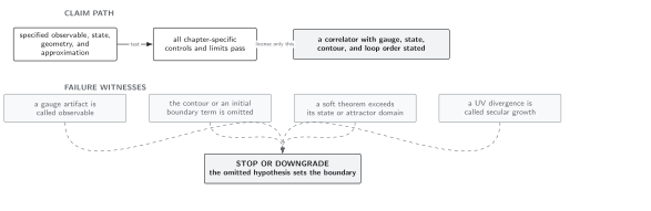
The accepted bispectrum is invariant under allowed integrations by parts and field redefinitions after all induced boundary and observable-map terms are included. Schematic; not to scale.

References

• Chen, X., M.-x. Huang, S. Kachru, and G. Shiu, “Observational Signatures and Non-Gaussianities of General Single Field Inflation,” Journal of Cosmology and Astroparticle Physics 01, 002 (2007), doi:10.1088/1475-7516/2007/01/002.
• Maldacena, J., “Non-Gaussian Features of Primordial Fluctuations in Single Field Inflationary Models,” Journal of High Energy Physics 05, 013 (2003), doi:10.1088/1126-6708/2003/05/013.