Why Interacting Curved-Space QFT Requires Local and Covariant Renormalization

Renormalization on an arbitrary curved spacetime must produce the same local observable whenever the local metric, couplings, and field configuration are the same. A prescription tied to a chart, a mode decomposition, or a preferred global state can remove a divergence, yet fail to define one quantum field theory across backgrounds. Local covariance turns that comparison requirement into a restriction on every Wick power, time-ordered product, and finite counterterm.

Required background. Local covariance and admissible embeddings supplies the background category and naturality condition; the Hadamard microlocal criterion controls products of singular distributions; and counterterm locality explains why ultraviolet changes are local.

Helpful background. Local composite insertions fixes the operator-valued-distribution viewpoint, while effective field theory as a controlled expansion clarifies how higher-dimension curvature terms are ordered.

Renormalized fields as natural local constructions

Consider a causality-preserving isometric embedding $\chi:(M,g)\to(M',g')$ whose image is causally convex. A locally covariant scalar composite $\mathcal O$ obeys

$$\alpha_\chi\!\left(\mathcal O_{(M,g)}(f)\right) =\mathcal O_{(M',g')}(\chi_*f),$$

where $f$ is supported in $M$ and $\alpha_\chi$ embeds the local observable algebra. This says more than coordinate covariance. The value inside $\operatorname{supp}f$ may depend on the germ of the metric and background couplings there, but not on how that region is embedded into a larger universe or on a state selected using the distant geometry.

For a free scalar, a Hadamard two-point function has the local form

$$\omega_2(x,x')=H_\mu(x,x')+W_\omega(x,x'),$$

where $H_\mu$ carries the universal geometric singularity and $W_\omega$ is smooth and state dependent. Point splitting defines

$$[\phi^2]_{\mu}(x) =\lim_{x'\to x}\bigl(\phi(x)\phi(x')-H_\mu(x,x')\mathbf 1\bigr),$$

with the limit understood distributionally. A second admissible prescription cannot add an arbitrary function of position. In four dimensions, covariance and scaling restrict the scalar ambiguity to

$$[\phi^2]'=[\phi^2]+c_m m^2\mathbf 1+c_R R\mathbf 1,$$

for dimensionless constants $c_m,c_R$ (and corresponding dependence on dimensionless couplings). This finite freedom is physical input to be fixed by renormalization conditions, not evidence that the field is undefined. Hollands and Wald prove the analogous finite local classification for Wick powers and time-ordered products under locality, covariance, scaling, continuity, and microlocal spectral conditions (Hollands and Wald 2001, Theorems 5.1–5.2).

Interacting fields inherit the same requirement. Renormalized time ordering must agree on causally ordered configurations, extend singular coefficients only on coincidence diagonals, and commute with admissible embeddings. The extension coefficients are consequently polynomials in the fields, masses, couplings, curvature, and their covariant derivatives, subject to dimension and symmetry. No momentum-space subtraction tied to a particular chart has that property automatically.

Four constraints and what each prevents

Locality. A counterterm at $x$ depends on a finite jet of the metric, fields, and background couplings at $x$. This prevents an ultraviolet subtraction from sampling remote boundaries or a global mode spectrum.

Covariance. The prescription is natural under admissible embeddings. This prevents two isometric neighborhoods from receiving different answers merely because they lie in different spacetimes.

Causal factorization. Changing an interaction in a region causally irrelevant to an observable changes its representative at most by the canonical local-algebra identification. This replaces an assumed global S-matrix with a local construction.

Microlocal admissibility. Products are formed only when their wavefront sets satisfy Hörmander’s criterion; renormalization extends the remaining singular distributions to diagonals without introducing forbidden covectors. This prevents formal Feynman expressions from hiding undefined products. The position-space construction on globally hyperbolic backgrounds is developed in Brunetti and Fredenhagen 2000, §§ 4–6.

Scaling supplements these constraints. Exact homogeneous scaling is usually spoiled by logarithms, but almost-homogeneous scaling bounds the extension freedom and organizes the renormalization group. Smooth or analytic dependence on the metric and parameters excludes discontinuous choices based on accidental spectral degeneracies.

The construction map locates the role of local covariance before any interacting observable is formed. Inspect the extension and checkpoint stages: a subtraction that cannot be transported between locally isometric backgrounds never reaches the local-S-matrix stage.

Local covariance is a condition on the first ultraviolet extension and therefore on every downstream observable. The construction is schematic and not to scale; the highlighted logical dependence does not assert a global switching limit.

For this page, the decisive failure witness is a nonlocal or chart-dependent counterterm. The lower map should be read as an embedding test: incompatible values in isometric regions force the claim back to a background-specific subtraction.

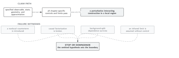
Failure path for a proposed renormalization prescription. This schematic, not-to-scale map shows why coordinate covariance or finiteness alone is insufficient: locality and embedding compatibility are decisive controls.

Application: two overlapping curved backgrounds

Let $U$ and $U'$ be isometric causally convex neighborhoods, related by $\chi:U\to U'$, and take a compactly supported test function $f\subset U$. Define the first-order interacting composite for $V=\int g\lambda\phi^4/4!$ by the retarded expansion

$$[\phi^2]_V(f) =[\phi^2](f)+\frac{i}{\hbar}R_1\!\left(V;[\phi^2](f)\right)+O(\lambda^2).$$

With locally covariant time-ordered products and $g=1$ on the causal neighborhood relevant to $f$,

$$\alpha_\chi\bigl([\phi^2]_{V,U}(f)\bigr) =[\phi^2]_{\chi_*V,U'}(\chi_*f)+O(\lambda^2).$$

Any difference between admissible schemes is the transported local combination $c_m m^2+c_RR$ plus the corresponding interacting finite redefinition. The comparison is reproducible once the metric germ, $m,\xi,\lambda$, switching function, perturbative order, and constants $c_m,c_R$ are stated. It does not require the two ambient spacetimes to share a vacuum.

Now regulate in coordinates by cutting off coordinate momenta, $|k_i|<\Lambda$, and subtract the coincident expectation value in a global vacuum $\Omega_M$. Repeating the recipe in $M'$ gives

$$\Delta(x)= \langle\phi^2(x)\rangle_{\Omega_M}^{\rm sub} -\langle\phi^2(\chi x)\rangle_{\Omega_{M'}}^{\rm sub}.$$

Even when the geometries agree on $U$, $\Delta$ generally contains smooth state-dependent terms because the two global vacua encode different exterior geometry. A coordinate cutoff also changes under a nonlinear chart transformation. Neither difference is forced to be $c_m m^2+c_RR$, so the construction fails the embedding test. The strongest surviving claim is only a chart-and-state-specific numerical subtraction on the chosen background; it is not a locally covariant composite.

Domain and failure conditions

The chapter-wide comparison is summarized in the domain and failure-conditions table. Here the assumptions are globally hyperbolic backgrounds, admissible causally convex embeddings, Hadamard microlocal behavior, and a finite-jet local prescription. They license a natural family of perturbative composites, unique only up to the stated local curvature terms. The decisive check is equality after transporting the observable between locally isometric regions. If a chart, exterior boundary, or global vacuum changes the subtraction inside such a region, the result must be downgraded to a prescription on that single background; the next valid handoff is to rebuild its time-ordered products by local diagonal extension.

Checks and limits

• In Minkowski spacetime with the standard vacuum, a locally covariant prescription can be normalized to agree with familiar normal ordering, but that normalization does not define normal ordering on every background.
• Changing the Hadamard state changes $\omega([\phi^2])$ through the smooth bisolution $W_\omega$; changing the renormalization prescription changes the operator by a state-independent local curvature term. These are distinct operations.
• Boundaries require boundary-compatible local data and can allow additional boundary counterterms. The interior classification above applies away from the boundary or when the boundary problem is separately specified.
• Local covariance constrains finite terms but does not choose their measured values. Renormalization conditions or matching do that.

Exercise

Show that the difference of two Hadamard-state expectations of the same locally covariant $[\phi^2]$ is independent of the finite constants $c_m,c_R$.

Solution

For states $\omega$ and $\omega'$, a scheme change gives $[\phi^2]'=[\phi^2]+(c_m m^2+c_RR)\mathbf1$. Therefore

$$\omega([\phi^2]')-\omega'([\phi^2]') =\omega([\phi^2])-\omega'([\phi^2]),$$

because both normalized states assign the same value to the identity. Equivalently, the difference is the coincidence limit of the smooth bisolution $W_\omega-W_{\omega'}$. State comparison is scheme independent even though each one-point function is not.

Handoff

The next step is to construct the renormalized time-ordered products whose finite changes generate these local ambiguities. That construction must distinguish distributions defined away from coincidence from their extensions to the diagonals.

References

• Brunetti, Romeo, and Klaus Fredenhagen. “Microlocal Analysis and Interacting Quantum Field Theories: Renormalization on Physical Backgrounds.” Communications in Mathematical Physics 208 (2000): 623–661. doi:10.1007/s002200050004.
• Hollands, Stefan, and Robert M. Wald. “Local Wick Polynomials and Time Ordered Products of Quantum Fields in Curved Spacetime.” Communications in Mathematical Physics 223 (2001): 289–326. doi:10.1007/s002200100540.
• Hollands, Stefan, and Robert M. Wald. “Quantum Fields in Curved Spacetime.” Physics Reports 574 (2015): 1–35. doi:10.1016/j.physrep.2015.02.001.