Bogoliubov Transformations and Unitary Implementability

A Bogoliubov transformation can preserve every canonical commutator and still have no unitary implementer on a chosen Fock space. For a bosonic pure quasifree representation, the decisive condition is that the transformation’s antilinear part be Hilbert–Schmidt. The subtle point is spatial homogeneity: in infinite volume, $\int \mathrm d^n k\,|\beta(\mathbf k)|^2/(2\pi)^n$ is a particle-number density, not the Hilbert–Schmidt norm of the diagonal continuum map. A finite density can therefore coexist with an extensive total number and globally inequivalent Fock representations.

Required background. Complex Structures and One-Particle Spaces defines the positive-frequency splittings being compared. Quasifree States and Two-Point Functions supplies their covariance data. Fock Space, Vacuum, and Particle Number fixes the number-operator conventions used below.

Helpful background. Unbounded Operators, Domains, Closure, and Adjoints explains why operator domains matter. Haag’s Theorem concerns a different route to inequivalent representations in interacting QFT.

Canonical mixing and its antilinear part

Let $\{u_i\}$ and $\{v_j\}$ be complete positive-norm mode families for the same real linear field, normalized with the conserved Klein–Gordon product. With one common convention,

$$v_j=\sum_i\left(\alpha_{ji}u_i+\beta_{ji}u_i^*\right), \qquad b_j=\sum_i\left(\alpha_{ji}^*a_i-\beta_{ji}^*a_i^\dagger\right).$$

Preserving the canonical commutation relations requires

$$\alpha\alpha^\dagger-\beta\beta^\dagger=1, \qquad \alpha\beta^{\mathsf T}=\beta\alpha^{\mathsf T}.$$

These equations say that the classical transformation is symplectic. They do not say that both particle descriptions live in the same Fock representation.

More invariantly, after choosing a one-particle Hilbert space $\mathcal H$, the transformation has a complex-linear part $A$ and a complex-antilinear part $B$. In the mode basis above, $B$ is represented by $\beta$ up to the displayed conjugations and sign convention. This distinction matters because unitary implementability tests $B$ as an operator, not merely the pointwise size of a function called $\beta_{\mathbf k}$.

The Shale criterion

For a bounded bosonic canonical transformation, a unitary $U$ on the original Fock space satisfying

$$b(f)=U\,a(f)\,U^{-1}$$

exists if and only if the antilinear part is Hilbert–Schmidt:

$$\lVert B\rVert_{\mathrm{HS}}^2 =\sum_r\lVert B e_r\rVert^2<\infty ,$$

where $\{e_r\}$ is any orthonormal basis of $\mathcal H$. This is the Shale theorem Shale 1962, Theorem 4.1, p. 157. In the equivalent complex-structure formulation, the corresponding difference of polarizations must be Hilbert–Schmidt after the one-particle norms have been identified Wald 1994, §4.4, Theorem 4.4.1, pp. 66–71.

When $B$ is Hilbert–Schmidt, the transformed number seen in the original vacuum is

$$\langle 0_a|N_b|0_a\rangle =\operatorname{Tr}(B^\dagger B) =\lVert B\rVert_{\mathrm{HS}}^2.$$

If the trace diverges, this formula is best read through finite-rank or finite-volume regulators: the regulated expectations grow without a finite limit, and the transformed vacuum is not a vector in the original Fock space.

The criterion just stated compares pure Fock representations. General quasifree states require a covariance criterion rather than the slogan “square-integrable beta”: the induced one-particle topologies must agree, and an appropriate difference of square-root covariance operators must be Hilbert–Schmidt Araki and Yamagami 1982, main theorem, PDF pp. 283–285.

Why a homogeneous continuum beta is not a Hilbert–Schmidt kernel

Consider a translation-invariant transformation on

$$\mathcal H=L^2\!\left(\mathbb R^n,\frac{\mathrm d^n k}{(2\pi)^n}\right)$$

whose antilinear part acts as

$$(Bf)(\mathbf k)=\beta(\mathbf k)\, \overline{f(-\mathbf k)}.$$

Writing this informally as a kernel proportional to $\beta(\mathbf k)\delta(\mathbf k+\mathbf k')$ can tempt one to replace the Hilbert–Schmidt norm by a single momentum integral. That would require squaring the delta distribution. The genuine operator is multiplication by $\beta$, composed with reflection and conjugation.

On the nonatomic space $L^2(\mathbb R^n)$, every nonzero bounded multiplication operator is noncompact. To see the obstruction directly, choose $\varepsilon>0$ so that

$$E_\varepsilon=\{\mathbf k:|\beta(\mathbf k)|\geq\varepsilon\}$$

has positive measure. Partition a finite-measure subset of $E_\varepsilon$ into infinitely many disjoint pieces, choose normalized functions $g_j$ supported on them, and set

$$f_j(\mathbf k)=\overline{g_j(-\mathbf k)}.$$

Reflection and conjugation preserve orthonormality, while

$$(Bf_j)(\mathbf k)=\beta(\mathbf k)g_j(\mathbf k).$$

The images have disjoint supports and norms at least $\varepsilon$. They have no convergent subsequence, so $B$ is not compact and therefore cannot be Hilbert–Schmidt.

Thus a nonzero homogeneous diagonal Bogoliubov transformation in infinite volume is not globally implementable, even when

$$\rho_\beta =\int\frac{\mathrm d^n k}{(2\pi)^n}\,|\beta(\mathbf k)|^2$$

is finite. The integral is physically useful—it is the particle-number density obtained from the thermodynamic limit—but it is not the global Shale norm.

Finite boxes and the thermodynamic limit

Keep these settings conceptually separate.

Setting	Implementability test	What a finite answer establishes
Finite set of modes	Every $B$ is finite rank.	Only the truncated model is unitarily implementable.
Fixed torus $T_L^n$, all momentum modes	$\sum_{\mathbf m\in\mathbb Z^n}\lvert\beta_{\mathbf m}\rvert^2<\infty$	The fixed-volume transformation is implementable if the zero mode is well defined and the ultraviolet sum converges.
Homogeneous $\mathbb R^n$ limit	The multiplication-reflection operator itself must be Hilbert–Schmidt.	Any nonzero homogeneous map fails globally, even if its density is finite.
Localized wavepacket mixing	Sum the squared singular values of the genuine integral kernel.	Finite rank, and more generally Hilbert–Schmidt mixing, is implementable.

A finite box alone is not a finite-mode truncation. It regulates volume and discretizes momentum but leaves infinitely many ultraviolet modes. Ultraviolet summability must be checked independently or imposed with a separate cutoff; the box size must be tracked when the thermodynamic limit is taken.

For an exact, ultraviolet-safe example in $n=3$, take

$$\beta_{\mathbf k} =b\,e^{-|\mathbf k|^2/(2\kappa^2)}, \qquad \alpha_{\mathbf k} =\sqrt{1+|\beta_{\mathbf k}|^2},$$

with real $b$ and $\kappa>0$. The even coefficients satisfy the canonical identities. On a cubic torus with $\mathbf k_{\mathbf m}=2\pi\mathbf m/L$, no ultraviolet mode cutoff is needed:

$$N_\beta(L) =b^2\sum_{\mathbf m\in\mathbb Z^3} \exp\!\left[-\frac{4\pi^2|\mathbf m|^2}{\kappa^2L^2}\right].$$

Poisson summation gives the independent exact form

$$\frac{N_\beta(L)}{L^3} =\rho_\infty \left[ \sum_{\boldsymbol\ell\in\mathbb Z^3} \exp\!\left(-\frac{\kappa^2L^2|\boldsymbol\ell|^2}{4}\right) \right], \qquad \rho_\infty=\frac{b^2\kappa^3}{8\pi^{3/2}}.$$

The bracketed factor tends exponentially to $1$, so

$$N_\beta(L)\sim \rho_\infty L^3 .$$

Every fixed-$L$ Gaussian transformation is implementable, its density approaches a finite limit, and its total transformed occupation nevertheless grows with the spatial volume. This is the finite-volume route to the same global obstruction proved above.

For a massive scalar in Minkowski space, with the flat tori above used only as regulators, both $\beta_{\mathbf k}$ and $\alpha_{\mathbf k}-1$ are rapidly decreasing. Every spacetime derivative of the two-point-function difference inserts only polynomial momentum weights, and the resulting Fourier integrands remain absolutely integrable. The difference from the Minkowski-vacuum two-point function is therefore a smooth bisolution, so the transformed pure quasifree state remains Hadamard. The mass assumption also avoids treating a massless torus zero mode as an ordinary oscillator. This example isolates global Fock inequivalence without introducing an ultraviolet singularity defect.

Ultraviolet and infrared thresholds

Density convergence remains an important, separate diagnostic. If

$$|\beta(k)|\sim k^{-r} \quad (k\to\infty),$$

then the radial ultraviolet integral behaves as

$$\int^\infty \mathrm dk\,k^{n-1-2r}$$

and converges exactly when $2r>n$. If instead

$$|\beta(k)|\sim k^{-s} \quad (k\to0),$$

the infrared integral converges exactly when $2s<n$. Equality in either condition gives a logarithmic divergence. These tests diagnose the density; passing them does not turn the homogeneous continuum operator into a Hilbert–Schmidt operator.

The figure separates those two questions. In the shell-weight panel, inspect whether the occupation per logarithmic momentum interval tends to zero or to a constant at either endpoint. In the volume panel, compare the exact torus sum with its Poisson-dual evaluation and the $L^3$ asymptote; the rank-one line is the implementable control.

On a narrow screen, swipe or use the Left and Right arrow keys to pan across the figure. Home and End move to its edges. A full-size link is also available.

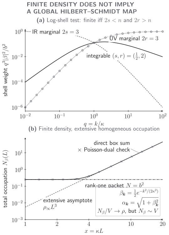
Finite particle density is not the Shale criterion for a translation-invariant continuum map. Exact direct and Poisson-dual torus sums approach the asymptotic law $N_\beta\sim\rho_\infty L^3$, while a rank-one wavepacket squeeze stays finite. The shell weights vanish at both endpoints only in the integrable case; a constant infrared or ultraviolet tail marks the logarithmic boundaries $2s=3$ and $2r=3$. Exact for the frozen data with $b=1/2$; the singular infrared control excludes the zero mode.

The machine-readable benchmark and CSV projection retain the direct and Poisson sums, continuum normalization, shell controls, and rank-one comparison.

A genuinely Hilbert–Schmidt contrast

Let $g\in\mathcal H$ be normalized and fixed by the chosen one-particle conjugation—the precise meaning of a real wavepacket here—and squeeze only that oscillator mode:

$$b(g)=\sqrt{1+b^2}\,a(g)-b\,a^\dagger(g), \qquad b(h)=a(h)\quad\text{for }h\perp g.$$

The antilinear operator has rank one and a single nonzero singular value $|b|$. Hence

$$\lVert B\rVert_{\mathrm{HS}}^2=b^2,$$

independent of the size of any surrounding box. This is not a homogeneous squeeze of every momentum mode. It acts only along a one-dimensional subspace of one-particle space, and Shale’s criterion correctly declares it implementable.

Local comparison without a global unitary

Global inequivalence does not imply that bounded-region measurements become incomparable. For the Klein–Gordon Weyl algebra with smooth real potential on a globally hyperbolic spacetime, the restrictions of any two quasifree Hadamard states to a relatively compact open region are quasiequivalent Verch 1997, Theorem 3.6(b), PDF pp. 28–30. The theorem has real hypotheses: quasifree states, the Hadamard condition, the stated field equation and spacetime setting, and localization to a relatively compact region. It is not a theorem about arbitrary states or unbounded regions.

Quasiequivalence means that the two restricted representations have the same normal state space; it does not provide one global unitary intertwining the full Fock representations. The Gaussian example above can therefore be locally well behaved and Hadamard while remaining globally inequivalent to the reference vacuum.

Where this test sits in the state construction

Bogoliubov coefficients compare two one-particle splittings. The canonical identities, the Shale test, the Hadamard condition, and physical state selection answer different questions. In the structure map, follow the representation branch without treating a passed commutator check as a passed ultraviolet or implementability check.

Canonical mode mixing preserves the CCR, while the Hadamard condition and global unitary implementability are separate tests. Schematic; not to scale.

The failure map records the necessary downgrade. Divergence during regulator removal ends the global unitary-equivalence claim, but it does not invalidate the canonical transformation or, under the hypotheses above, local quasiequivalence.

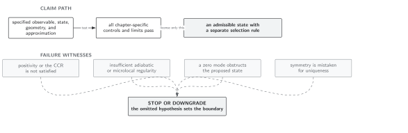
Regulator removal fixes the scope of the implementability claim: divergence removes global Fock-space equivalence without disproving the CCR relation or every local comparison. Schematic; not to scale.

For the chapter-wide distinction among canonical, ultraviolet, global, and local claims, see Domain and failure conditions.

Common pitfalls

Calling the density the Shale norm. The integral over one momentum variable is the thermodynamic particle density for a homogeneous state. The continuum beta kernel also contains momentum conservation; the resulting multiplication-reflection operator is noncompact whenever it is nonzero.

Calling a finite box finite dimensional. A torus has discrete but infinitely many momentum modes. Implementability at fixed $L$ still requires ultraviolet summability unless a separate mode cutoff is imposed.

Checking only the ultraviolet. A rapidly decaying high-momentum tail can coexist with an infrared divergence. Test both endpoints, including the zero-mode prescription.

Equating global inequivalence with different local physics. Global particle number and local normality are different diagnostics. Apply a local theorem only after verifying its spacetime, field, state-class, and region hypotheses.

Exercises

Show that the mode transformation preserves $[b_i,b_j^\dagger]=\delta_{ij}$ and $[b_i,b_j]=0$ precisely when the two displayed canonical identities hold.

Solution

Insert

$$b_j=\sum_i\left(\alpha_{ji}^*a_i-\beta_{ji}^*a_i^\dagger\right)$$

and use $[a_i,a_\ell^\dagger]=\delta_{i\ell}$. The mixed commutator becomes

$$[b_j,b_\ell^\dagger] =(\alpha^*\alpha^{\mathsf T}-\beta^*\beta^{\mathsf T})_{j\ell},$$

which is the complex conjugate of $\alpha\alpha^\dagger-\beta\beta^\dagger=1$. The annihilation–annihilation commutator is

$$[b_j,b_\ell] =-\sum_i\left(\alpha_{ji}^*\beta_{\ell i}^* -\beta_{ji}^*\alpha_{\ell i}^*\right),$$

and vanishes by the complex conjugate of the second identity.

Derive the ultraviolet and infrared density thresholds in $n$ spatial dimensions.

Solution

After angular integration, the density is proportional to

$$\int_0^\infty \mathrm dk\,k^{n-1}|\beta(k)|^2.$$

For $|\beta|\sim k^{-r}$ at infinity, the integrand is $k^{n-1-2r}$, whose upper endpoint converges when $n-1-2r<-1$, or $2r>n$. For $|\beta|\sim k^{-s}$ at the origin, convergence requires $n-1-2s>-1$, or $2s<n$. Equality gives $\int \mathrm dk/k$ and is logarithmic.

Use one-dimensional Poisson summation to derive the Gaussian finite-volume formula and its continuum density.

Solution

For $a>0$,

$$\sum_{m\in\mathbb Z}e^{-a m^2} =\sqrt{\frac{\pi}{a}} \sum_{\ell\in\mathbb Z}e^{-\pi^2\ell^2/a}.$$

Taking $a=4\pi^2/(\kappa^2L^2)$ and cubing the result gives

$$N_\beta(L) =b^2\left(\frac{\kappa L}{2\sqrt{\pi}}\right)^3 \left[ \sum_{\ell\in\mathbb Z}e^{-\kappa^2L^2\ell^2/4} \right]^3.$$

Therefore

$$\frac{N_\beta(L)}{L^3} =\frac{b^2\kappa^3}{8\pi^{3/2}} \left[ \sum_{\ell\in\mathbb Z}e^{-\kappa^2L^2\ell^2/4} \right]^3 \longrightarrow \frac{b^2\kappa^3}{8\pi^{3/2}}.$$

Prove that the homogeneous multiplier is non-Hilbert–Schmidt while the one-wavepacket squeeze has Hilbert–Schmidt norm squared $b^2$.

Solution

If the multiplier is nonzero, there is an $\varepsilon>0$ and a positive-measure set $E_\varepsilon$ on which $|\beta|\geq\varepsilon$. Choose normalized $g_j$ on infinitely many disjoint subsets of $E_\varepsilon$ and define $f_j(\mathbf k)=\overline{g_j(-\mathbf k)}$. Then $(Bf_j)(\mathbf k)=\beta(\mathbf k)g_j(\mathbf k)$, so the images have disjoint supports and norm at least $\varepsilon$. The image sequence has no convergent subsequence. The operator is not compact; every Hilbert–Schmidt operator is compact.

For the wavepacket squeeze, the antilinear operator vanishes on $g^\perp$ and maps the normalized vector $g$ to a vector of norm $|b|$. Its singular values are therefore $|b|,0,0,\ldots$, and their squared sum is $b^2$.

Handoffs

GNS Representations, Local Normality, and Local Quasiequivalence develops the local comparison. Dynamical production rates belong to Particles, Detectors, and Nonadiabatic Production. Proof-level representation theory continues in States, GNS Representations, and Folia.

References

• Araki, Huzihiro, and Shigeru Yamagami. “On Quasi-Equivalence of Quasifree States of the Canonical Commutation Relations.” Publications of the Research Institute for Mathematical Sciences 18 (1982): 283–338. DOI; Open PDF.
• Shale, David. “Linear Symmetries of Free Boson Fields.” Transactions of the American Mathematical Society 103 (1962): 149–167. DOI.
• Verch, Rainer. “Continuity of Symplectically Adjoint Maps and the Algebraic Structure of Hadamard Vacuum Representations for Quantum Fields on Curved Spacetime.” Reviews in Mathematical Physics 9 (1997): 635–674. DOI; Open PDF.
• Wald, Robert M. Quantum Field Theory in Curved Spacetime and Black Hole Thermodynamics. Chicago Lectures in Physics. Chicago: University of Chicago Press, 1994. Publisher.