de Sitter Infrared Regimes: States, Observables, Gauges, and Limits

An infrared statement in de Sitter is a statement about a specified distribution or observable in a specified state and patch, with a declared regulator and limit order. A growing coordinate two-point function, a finite local composite, a detector response, and a relational gravitational observable can legitimately behave differently.

Required background. Bunch–Davies and alpha-state diagnostics fixes the free-state classes, and state-selection failure modes fixes admissibility tests. Helpful background. Review secular resummation, cosmological initial states, and cosmological loops.

The infrared claim tuple

For a scalar in four-dimensional exact de Sitter, record

$$\mathcal C=(\mathcal P,\omega,\mathcal O,\mathcal G, \mathcal R,\mathcal L,\Delta t),$$

where $\mathcal P$ is the patch, $\omega$ the state, $\mathcal O$ the observable, $\mathcal G$ any gauge or dressing, $\mathcal R$ the regulator/subtraction, $\mathcal L$ the ordered limits, and $\Delta t$ the duration. Two calculations disagree physically only after these entries are translated.

For $P=\Box+m^2+\xi R$ in the site’s convention, define $M^2=m^2-12\xi H^2$. The light massive Euclidean/BD field has $\nu^2=9/4-M^2/H^2$ and long-mode decay exponent

$$\Delta_-=\frac32-\nu \simeq\frac{M^2}{3H^2}.$$

At fixed comoving point, the leading long variance accumulated after $t_0$ is

$$\langle\phi_L^2(t)\rangle \simeq\frac{3H^4}{8\pi^2M^2} \left[1-e^{-2M^2(t-t_0)/(3H)}\right].$$

Consequently,

$$\lim_{M\to0}\langle\phi_L^2(t)\rangle =\frac{H^3(t-t_0)}{4\pi^2}, \qquad \lim_{t\to\infty}\langle\phi_L^2(t)\rangle =\frac{3H^4}{8\pi^2M^2}.$$

The massless and late-time limits do not commute. The infinite-volume limit adds a third possible obstruction because the homogeneous sector is treated differently on compact global slices and in a planar-patch momentum integral.

The underlying free-state classification already separates the ordinary massive Euclidean family from the minimally coupled zero-mode obstruction Allen 1985, §§II–IV, pp. 3138–3147.

First application: classify a massive spectator

Take $0<M^2\ll H^2$ in the Euclidean/BD state and compare four objects: the Wightman function at invariant separation, an equal-comoving-point long variance, the local point-split $\langle\phi^2\rangle_{\rm ren}$, and a derivative correlator. State whether separation is held at fixed physical distance, fixed comoving distance, or fixed de Sitter invariant $Z$. The first decays at large invariant separation for $M^2>0$; the second grows until the relaxation time; the local composite includes a scheme-dependent local curvature ambiguity; derivatives suppress the constant infrared sector.

This classification explains why massive Euclidean-state stability results do not automatically extend to the minimally coupled zero mode. Perturbative massive scalar correlators in the Euclidean state have controlled large-separation behavior under explicit hypotheses Hollands 2013, Theorems 1–2 and §§5–6, pp. 27–53. The hypothesis that the free Euclidean state exists is decisive.

Now compare two interactions. A shift-symmetric derivative interaction inserts momenta on soft lines and can remove the leading constant mode from local derivative observables. A non-shift-symmetric light potential interaction acts directly on that mode and can produce powers of $\ln a$ at fixed order. The two theories do not share one infrared power count merely because their free propagators use the same coordinates.

The structure map places this tuple before every resummation or stochastic claim. Inspect the branches separating scalar field correlators, local composites, and relational graviton quantities.

Infrared behavior belongs to a complete claim tuple; different correlators and local or relational observables need not share the same long-distance limit. Schematic; not to scale.

Domain and failure conditions

Use the chapter’s canonical domain table. The displayed variance is a leading light-field, fixed-$H$, long-wavelength expression; it is not the full renormalized coincidence limit. Patch restrictions, initial transients, ultraviolet subtraction, and the spatial coarse-graining window remain separate data.

Adversarial test. Exchange the $M\to0$, volume, and $t\to\infty$ limits. Repeat with a small mass and a finite comoving box, then compare the same derivative or shift-invariant observable after removing each regulator. Apply the exercise separately to a derivative interaction and a light potential interaction. Reject universal growth, instability, or stochastic claims whenever regulator-independent agreement survives only for a narrower observable class.

The validity map identifies precisely where a limit swap or observable substitution changes the conclusion. A controlled scalar claim passes to free-field construction, zero-mode analysis, or interacting logarithms with the full tuple attached.

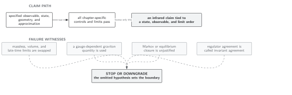
Noncommuting limits and object-dependent soft behavior require the conclusion to be narrowed to the exact state, regulator, and observable that passed comparison. Schematic; not to scale.

References

• Allen, B., “Vacuum States in de Sitter Space,” Physical Review D 32, 3136–3149 (1985), doi:10.1103/PhysRevD.32.3136.
• Hollands, S., “Correlators, Feynman Diagrams, and Quantum No-Hair in de Sitter Spacetime,” Communications in Mathematical Physics 319, 1–68 (2013), doi:10.1007/s00220-012-1653-2.