

Quantum-State Evolution on Backreacted Backgrounds
A backreacted evolution is a coupled history: the state determines the renormalized stress tensor, that stress changes the geometry, and the changed geometry in turn changes the field equation and the state’s propagation. The invariant object to evolve is a state on the local field algebra—often represented by its two-point function—not an instantaneous particle number. This page formulates that coupling for a Gaussian scalar state on a homogeneous spacetime and identifies the checks that keep the result causal, Hadamard, and constraint consistent.
Required background. Self-consistent state–geometry solutions supplies the coupled fixed-point problem; propagation of the Hadamard property supplies ultraviolet regularity under hyperbolic evolution; and initial density matrices on the closed time path supplies the state data for causal expectation values.
Helpful background. Adiabatic states and WKB order gives a practical homogeneous-state parametrization, while particle observables and detector dependence explains why particle number is not the state itself.
Coupled propagation of geometry and correlations
Section titled “Coupled propagation of geometry and correlations”Take a spatially flat FLRW line element
and a real scalar satisfying the site convention
For a homogeneous Gaussian state, write
where occupation and pairing data can be incorporated in the initial two-point function. The modes obey
The Wronskian is the mode form of the canonical commutator; its conservation is therefore a non-negotiable numerical check. Equivalently, the evolved two-point function must retain
because this volume defines and .
At each time, the renormalized stress is obtained from the same state and metric,
with all finite local curvature terms fixed in one prescription. The mean equations then include
Here denotes the declared curvature-squared contributions. Evolving the modes on a prescribed and inserting their stress only afterward is a fixed-background calculation, not a self-consistent solution.
The coupled dependencies are worth seeing explicitly: state data feed the mean stress, while the constrained metric determines the next hyperbolic propagator. Inspect the central loop and the Bianchi checkpoint in the following map.

Coupled state–geometry evolution. The map is schematic and not to scale; the Wronskian, Hadamard property, stress conservation, and gravitational constraint must be checked along the loop rather than only at the final time.
A slowly backreacting homogeneous application
Section titled “A slowly backreacting homogeneous application”Choose fourth-order adiabatic initial data at for each , together with and satisfying the renormalized energy constraint. A practical causal step from to is:
- propagate the mode functions with the metric known through ;
- form the subtracted mode sums for and using the same subtraction convention;
- update the metric through the constraint and evolution equations; and
- iterate the step until the state and metric agree to the requested tolerance.
The adiabaticity parameters
diagnose a WKB representation; they do not by themselves measure the error in the backreacted metric. That error also contains finite-renormalization, mode-cutoff, time-step, iteration, and EFT-truncation contributions. Hadamard propagation says that smooth evolution from Hadamard initial data preserves the singularity class while the background remains globally hyperbolic (Fulling, Sweeny, and Wald 1978, pp. 257–264). It does not guarantee that a numerical truncation preserves the required high-frequency coefficients.
An operational comparison makes the distinction from particles sharp. Diagonalize the Hamiltonian at a time in two canonical variables—for example, and . The corresponding instantaneous Bogoliubov coefficients and occupation numbers generally differ. Nevertheless, if both are merely two representations of the same evolved and the same local subtraction prescription is used, they give the same . A disagreement in the local stress exposes a state, subtraction, or numerical mismatch; a disagreement only in instantaneous particle number need not.
Memory, causality, and the adversarial particle test
Section titled “Memory, causality, and the adversarial particle test”For interacting or effectively integrated-out matter, the source at need not be a function only of . A causal in-in equation has the form
so the initial density matrix and past geometry are part of the data. Replacing the retarded kernel by a Feynman kernel changes the problem into an in-out matrix element and can make a real initial-value problem complex or acausal.
The decisive adversarial test is to compute two different instantaneous particle numbers on the same numerical history. If they disagree while the renormalized local stress, Wronskian, conservation residual, and metric constraint agree within their independently converged errors, the ambiguity is harmless. Feeding either particle number back as though it were the source would manufacture prescription-dependent geometry.
The failure paths in the next map should be read as tests on the history, not as labels attached after a run. In particular, solving state and geometry in separate one-way passes misses the defining fixed point.
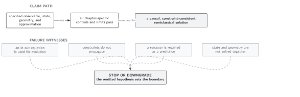
Validity and failure conditions for evolving a state on a changing mean geometry. The diagram is schematic and not to scale; particle-number agreement is deliberately absent because local renormalized observables, causal support, and constraints are the relevant tests.
Domain and failure conditions
Section titled “Domain and failure conditions”See the chapter domain and failure-conditions table. This construction assumes globally hyperbolic evolution, Hadamard initial data, a fixed finite-renormalization prescription, a causal in-in source, and a controlled derivative expansion. It must be downgraded if the ultraviolet tail ceases to match the subtraction, if constraint or Wronskian residuals fail to converge, if memory is replaced by instantaneous state data, or if the evolution reaches curvature or frequency scales comparable to the EFT cutoff.
Exercise
Section titled “Exercise”Show directly that the mode Wronskian is constant.
Solution
Differentiate and use the mode equation and its complex conjugate. The frequency terms cancel, while the two friction terms give
Multiplication by cancels this term because . The initial normalization therefore remains .
References
Section titled “References”- Fulling, S. A., M. Sweeny, and R. M. Wald. “Singularity Structure of the Two-Point Function in Quantum Field Theory in Curved Spacetime.” Communications in Mathematical Physics 63 (1978): 257–264. DOI.
- Parker, L., and D. Toms. Quantum Field Theory in Curved Spacetime: Quantized Fields and Gravity. Cambridge University Press, 2009. DOI.
- Wald, R. M. Quantum Field Theory in Curved Spacetime and Black Hole Thermodynamics. University of Chicago Press, 1994. Publisher.
Original QFT.org content:CC BY 4.0, unless an item supplies different terms. Third-party material retains its own terms.