Surface Charges, Integrability, and Ambiguities

A finite surface-charge variation is not yet a charge. On each connected component of the declared phase space, a Hamiltonian charge $H_\epsilon$ exists precisely when the surface one-form $\eta_\epsilon$ is globally exact. Local closure is necessary, vanishing periods supply the global test, and a reference configuration fixes only the remaining additive constant. Finiteness, conservation between cuts, and independence from improvement choices are separate requirements.

This page develops those tests for gauge theories on regions with boundary.

Required background. Proper and Improper Gauge Transformations establishes admissibility, completes the generator, and forms the finite null/non-null pairing. Presymplectic Systems and the Covariant Phase-Space Ambiguity Map constructs $\Omega_\Sigma$ and $\boldsymbol k_\epsilon$ and distinguishes boundary pairing, lateral flux, and corner-representative dependence.

Helpful background. Symplectic Forms, Hamiltonian Flows, and Poisson Brackets develops closed versus exact one-forms, global periods, and additive constants. Classical Symmetries, Currents, and Stress Tensors develops localized currents, boundary flux, and improvement freedom.

The main construction first keeps the gauge parameter fixed and field-independent. A later section states the extra prescription required when the parameter depends on the fields. Infinite-dimensional manifold theorems and gravitational charge formulae lie outside this page’s scope.

Surface-charge existence and conservation

Let $\mathcal P_0$ be one connected component of the constraint or solution space, with its admitted tangent variations. Fix a spatial hypersurface $\Sigma$ with boundary $S=\partial\Sigma$, and let $R_\epsilon$ be the field-space vector generated by an admissible parameter. The complete presymplectic form produces

$$\begin{aligned} \eta_{\epsilon,S}(\delta) &:= \bigl(\iota_{R_\epsilon}\Omega_\Sigma\bigr)(\delta)\\ &\mathrel{\widehat{=}} \int_S \boldsymbol k_\epsilon[\delta\Phi;\Phi]. \end{aligned}$$

Here $\mathrel{\widehat{=}}$ means equality after imposing the equations, linearized equations, constraints, and boundary conditions used to define $\mathcal P_0$. The object $\boldsymbol k_\epsilon$ has spacetime degree $d-2$ and field-space degree one. The decision has six distinct gates:

Existence, prescription, normalization, and conservation are separate gates

Question	Test	What a pass establishes
Is its prescription fixed?	Fix the symplectic-potential and corner representative, or explicitly carry its dependence.	The tested one-form and its prescription dependence are declared.
Is the candidate defined?	ηε,S is finite and is a genuine one-form on every admitted tangent direction.	A finite, well-defined candidate generator one-form exists.
Is it locally integrable?	δηε,S = 0.	A local primitive exists wherever the chosen field-space setting satisfies the Poincaré lemma.
Is it globally integrable?	∮Γηε,S = 0 for every closed field-space loop Γ in 𝒫0.	The path integral defines a single-valued Hε on 𝒫0.
Is its numerical value fixed?	Choose a reference in each connected component after exactness is established.	The additive constant is fixed.
Is it conserved?	Compare two cuts using the lateral presymplectic flux.	Hε is cut-independent or obeys a stated balance law.

The representative gate precedes closure, while the reference gate follows global exactness. A divergent or ill-defined expression cannot be made integrable by choosing a reference. Likewise, an integrable charge need not be conserved, and a conserved one need not be independent of a corner improvement.

Inputs, output, and practical difficulty

The calculation is reproducible only when the following inputs are stated.

Inputs that must be declared before testing a surface charge

Input	What must be fixed
Boundary phase space	Action including boundary and corner terms, fields, boundary conditions, equations or constraints, and admitted tangent variations.
Transformation	Parameter class, action of Rε, admissibility conditions, and whether ε is field-independent.
Presymplectic prescription	The complete Θ, ω, and ΩΣ, including required boundary or corner contributions.
Geometry	Orientation of Σ, S, and any lateral boundary, together with falloff or regularity assumptions.
Global sector	The connected component of field space, its relevant loops, and the reference configuration.

The output is either a finite reference-normalized function $H_\epsilon$, possibly accompanied by a flux balance law and a declared improvement dependence, or a precise stop reason. Extracting a local surface expression is often the shortest step. Testing closure requires two independent variations; testing periods can require the global topology of field space; and comparing representatives requires boundary and corner data. The global and representative tests are therefore usually the expensive parts.

Step 1: extract the surface one-form

With the site’s sign convention,

$$\boldsymbol\omega =-\boldsymbol\delta\boldsymbol\Theta, \qquad \Omega_\Sigma =-\boldsymbol\delta\Theta_\Sigma.$$

Write $\Omega_\Sigma$ for the complete form selected by the bounded variational problem, not automatically the integral of a bare bulk current. After the bulk constraints and linearized constraints have been used, a local gauge identity commonly reduces its contraction to $S$:

$$\iota_{R_\epsilon}\Omega_\Sigma \mathrel{\widehat{=}} \int_S\boldsymbol k_\epsilon.$$

This identity must be evaluated on the same phase space used to decide admissibility. Terms that vanish for compactly supported variations may survive at $S$; discarding them would erase the candidate charge. Conversely, adding an arbitrary boundary term after the calculation would change the prescription. Boundary conditions and the symplectic potential therefore belong upstream of the exactness test, as emphasized in Harlow and Wu 2020, §§ 2.1–2.4, pp. 7–23, Open PDF.

Step 2: require finiteness and differentiability

For every $\Phi\in\mathcal P_0$ and every admitted tangent $\delta\Phi$, $\eta_{\epsilon,S}(\delta)$ must be finite, linear in $\delta\Phi$, and compatible with the chosen regularity. A candidate also fails here if its value depends on an arbitrary extension of boundary data into the bulk, if an uncanceled variation remains outside the declared tangent space, or if $R_\epsilon$ does not preserve the boundary conditions.

This is differentiability of the proposed generator. It is not yet integrability: differentiability says that $\eta_\epsilon$ is a legitimate one-form; integrability asks whether that one-form is the differential of a function. Barnich and Compère keep finiteness, integrability, and conservation as distinct requirements in their asymptotic construction Barnich and Compère 2008, § 4.1, pp. 13–14, Open PDF.

Step 3: test local closure

For any field-space vector fields $\delta_1$ and $\delta_2$,

$$\begin{aligned} (\boldsymbol\delta\eta_\epsilon)(\delta_1,\delta_2) ={}& \delta_1\!\left[\eta_\epsilon(\delta_2)\right] -\delta_2\!\left[\eta_\epsilon(\delta_1)\right]\\ &-\eta_\epsilon([\delta_1,\delta_2]). \end{aligned}$$

Coordinate variations commute, but the commutator term is part of the definition and cannot be omitted for general vector fields. Exactness would give

$$\eta_\epsilon=\boldsymbol\delta H_\epsilon \quad\Longrightarrow\quad \boldsymbol\delta\eta_\epsilon=0,$$

so nonclosure is an immediate obstruction. In a contractible finite-dimensional chart, closure is locally sufficient by the Poincaré lemma. Applying the same statement to an infinite-dimensional solution space requires a chosen functional-analytic setting; here closure is used as the standard local diagnostic, not as an unqualified theorem about every space of fields. The finite-dimensional closed-versus-exact distinction and Poincaré lemma are reviewed in Frankel 2011, §§ 5.2 and 5.4, pp. 156–160.

Step 4: test periods and choose a reference

A closed one-form can still fail to be globally exact. The remaining test is

$$\boxed{ \oint_\Gamma\eta_\epsilon=0 \quad \text{for every closed loop }\Gamma\subset\mathcal P_0. }$$

When closure and the period test both pass, choose a path $\gamma:\bar\Phi\to\Phi$ within $\mathcal P_0$ and define

$$H_\epsilon[\Phi;\bar\Phi] = H_\epsilon[\bar\Phi] +\int_\gamma\eta_\epsilon.$$

The result is path-independent. On a simply connected component, closure and the usual regularity assumptions imply the period condition; otherwise the periods must be checked. This local-versus-global distinction and the path-integrated construction are developed in Wald and Zoupas 2000, § 3, pp. 9–12, Open PDF and Barnich and Compère 2008, § 3.4, pp. 11–13, Open PDF.

Setting $H_\epsilon[\bar\Phi]=0$ is a normalization, not an integrability argument. It cannot cure nonclosure, a nonzero period, a divergence, or an unfixed corner representative. Disconnected components admit independent constants because no path in field space compares their references.

A minimal global obstruction is the one-form $\eta=k\,\mathrm d\theta$ on a circle. It is closed, but $\oint_{S^1}\eta=2\pi k$. For $k\ne0$, no single-valued real function on $S^1$ has differential $\eta$.

Step 5: compare improvements and corner representatives

The working representative was fixed before Step 1. This step compares it with other admissible representatives; whenever the comparison changes $\eta_\epsilon$, Steps 2–4 must be repeated. The prerequisite ambiguity map permits

$$\boldsymbol\Theta' = \boldsymbol\Theta +\boldsymbol\delta\boldsymbol\ell +\mathrm d\boldsymbol\beta.$$

For the field-space one-form

$$B_S:=\int_S\boldsymbol\beta,$$

the complete presymplectic form changes by

$$\Omega_\Sigma' = \Omega_\Sigma -\boldsymbol\delta B_S.$$

Holding $R_\epsilon$ fixed and using the field-space Cartan identity gives the exact transformation law

$$\boxed{ \eta_\epsilon' = \eta_\epsilon -\mathcal L_{R_\epsilon}B_S +\boldsymbol\delta \bigl(\iota_{R_\epsilon}B_S\bigr). }$$

If $B_S$ is invariant under $R_\epsilon$, the shift is exact. It changes an integrated charge by the generally state-dependent corner functional $\iota_{R_\epsilon}B_S$; it is not necessarily an additive constant. If $B_S$ is not invariant, even the closure and integrability test can change. This is why a surface charge becomes convention-independent only relative to a declared class of admissible representatives for which the physical comparison is invariant, or after a physical boundary prescription selects one representative. There is no universal representative-independent number before that input is supplied.

These distinctions prevent several common substitutions:

Reference, representative, and phase-space changes have different effects

Change	Effect on the charge problem
Hε → Hε + Cε on one connected component	Changes the reference value but leaves ηε unchanged.
Invariant potential improvement BS	Preserves exactness but can shift Hε by a state-dependent corner functional.
Noninvariant or unfixed corner representative	Can change the local integrability test itself.
𝑳 → 𝑳 + dℓ	Leaves the compatible local presymplectic current ω unchanged but may alter the boundary action and admitted phase space.
New boundary conditions or edge variables	Defines a different phase space; it is not merely a convention change.

If the cut $S$ has its own boundary, spacetime-exact improvements on $S$ can leave lower-codimension corner terms. Their composition belongs with the charge-algebra and corner analysis on the next page.

Field-dependent parameters need an adjusted variation

Suppose $\epsilon=\epsilon[\Phi]$ varies smoothly with the fields and the charge family is linear in its parameter. The ordinary total variation of $H_{\epsilon[\Phi]}$ includes both the change of the fields and the change of the label. Define the fixed-label, or adjusted, variation by

$$\boxed{ \boldsymbol\delta_{\!\Phi}H_{\epsilon[\Phi]} := \boldsymbol\delta H_{\epsilon[\Phi]} -H_{\boldsymbol\delta\epsilon}. }$$

The surface one-form is compared with $\boldsymbol\delta_{\!\Phi}H_\epsilon$, not blindly with the total variation. Equivalently, its adjusted closure condition contains the parameter-variation terms

$$\begin{aligned} 0={}& \delta_1[\eta_\epsilon(\delta_2)] -\delta_2[\eta_\epsilon(\delta_1)] -\eta_\epsilon([\delta_1,\delta_2])\\ &-\eta_{\delta_1\epsilon}(\delta_2) +\eta_{\delta_2\epsilon}(\delta_1). \end{aligned}$$

This formula assumes a smooth parameter family, linearity in $\epsilon$, and a fixed reference prescription. Field dependence is not automatically an integrability obstruction; omitting $H_{\boldsymbol\delta\epsilon}$ can manufacture one. The subtraction term is explicit for internal gauge parameters in Speziale 2026, p. 26, footnote 11, Open PDF and for field-dependent diffeomorphisms in Speziale 2026, § 3.4, p. 30, eq. (3.60), Open PDF. The expanded adjusted-closure formula above is the exterior-calculus consequence of that subtraction under the stated smoothness, linearity, and fixed-transport assumptions; it is not quoted verbatim from those formulas. Around a field-space loop, $\epsilon$ must be transported consistently. Any holonomy or curvature of that transport is additional data and cannot be hidden inside an ordinary period test. The adjusted bracket and its extension terms are deferred to Charge Algebras, Central Terms, and Corners.

Step 6: separate conservation from integrability

Let $\Sigma_1$ and $\Sigma_2$ bound a spacetime slab whose lateral boundary is $B_{12}$, with cuts $S_i=\partial\Sigma_i$. Return first to a fixed, field-independent $\epsilon$ and transport that same parameter and representative between the cuts. Denote the complete lateral presymplectic flux by $\mathcal W^{\mathrm{comp}}_{B_{12}}$. On solutions and linearized solutions, the orientation convention defines it through

$$\Omega_{\Sigma_2}-\Omega_{\Sigma_1} = -\mathcal W^{\mathrm{comp}}_{B_{12}}.$$

When the complete hypersurface form has no additional boundary or corner contribution, $\mathcal W^{\mathrm{comp}}_{B_{12}}$ reduces to $\int_{B_{12}}\boldsymbol\omega$. In general it includes the lateral completion selected by the bounded variational problem. Contracting gives

$$\eta_{\epsilon,S_2}-\eta_{\epsilon,S_1} = -\iota_{R_\epsilon} \mathcal W^{\mathrm{comp}}_{B_{12}}.$$

If the contracted lateral flux is itself an exact field-space one-form, define a scalar flux by

$$\boldsymbol\delta\mathcal F_\epsilon[B_{12}] = \iota_{R_\epsilon} \mathcal W^{\mathrm{comp}}_{B_{12}}.$$

Compatible reference choices then give the balance law

$$\boxed{ H_\epsilon[S_2]-H_\epsilon[S_1] +\mathcal F_\epsilon[B_{12}]=0. }$$

For a field-dependent $\epsilon[\Phi]$, both the cut one-form and the scalar flux require the adjusted variation and a declared rule for transporting the parameter family between cuts. The ordinary-$\boldsymbol\delta$ formula above must not be reused unchanged.

Thus zero flux implies conservation, while nonzero controlled flux gives a balance law rather than a pathology. A charge can be integrable on every cut and still change between cuts. Conversely, a nonintegrable cut one-form is not repaired merely by calling its obstruction “flux.” Wald and Zoupas give a distinguished prescription for asymptotic gravitational radiation under additional hypotheses Wald and Zoupas 2000, § 4, pp. 12–19, Open PDF; it is an important example, not a universal finite-boundary repair.

The chapter-wide decision map

The diagram records the complete chapter sequence. Enter this page after a finite candidate one-form has been formed. This page fixes or tracks its representative, distinguishes the null, globally exact, and nonexact outcomes, treats the field-dependent-parameter caution, and tests flux. Charge brackets and optional edge extensions remain forward steps.

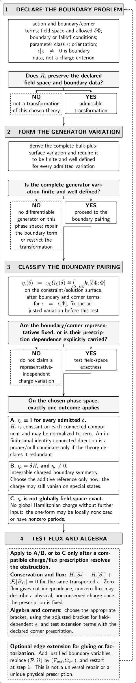
After admissibility and finiteness, a fixed representative supplies $\eta_\epsilon$. A vanishing one-form is a null candidate; a nonzero one-form defines a Hamiltonian charge only after local closure and global periods have been tested. Reference normalization follows exactness. Conservation and algebra are separate tests, and an edge extension replaces the phase space and restarts the classification. In the displayed convention, positive $\mathcal F_\epsilon[B_{12}]$ lowers $H_\epsilon$ from $S_1$ to $S_2$. The diagram is schematic and not to scale.

The complete text equivalent is:

Every gate, outcome, qualification, and restart in the decision map

Stage	Required test	Valid conclusion	Scope
Declare	Fix the action and boundary/corner terms, fields, admitted variations, boundary conditions, parameter class, and orientation.	The boundary problem is defined.	Prerequisite page; carried as input here.
Admit	Check that Rε preserves every declared datum.	Admissible, or else not a transformation of this theory.	Prerequisite page.
Form the generator	Derive the complete bulk-plus-surface variation and require it to be finite and well defined for every admitted variation.	A candidate generator one-form exists, or the construction stops.	Prerequisite page and Steps 1–2.
Fix representatives	Fix the symplectic-potential, improvement, and corner representatives, or carry their dependence.	The candidate has a declared prescription.	Input to Step 1; alternatives compared in Step 5.
Null outcome	Test ηε(δ) = 0 for every admitted δ.	The generator is componentwise constant; an identity-connected direction may be declared proper.	Prior classification, confirmed here.
Charged outcome	Test whether ηε = δHε globally, with ηε not identically zero.	An integrable charged boundary symmetry.	Steps 3–4.
Nonexact outcome	Test local closure and periods on field space.	No global Hamiltonian charge without further input.	Steps 3–4 and the stop rules below.
Field-dependent parameter	Define the adjusted variation before any of the three outcomes.	Field dependence changes the prescription, not the list of outcomes.	Adjusted-variation section.
Flux and algebra	For an existing or repaired charge, test Hε[S2] − Hε[S1] + ℱε[B12] = 0 and then the appropriate bracket.	Integrability alone establishes neither conservation nor a charge-algebra representation.	Flux here; algebra on the next page.
Optional extension	Justify new boundary variables, replace (𝒫, Ω) by (𝒫ext, Ωext), and restart.	An extension may solve a specified gluing problem; it is not universal.	Edge-mode page.

Worked application: relative Maxwell fluxes

Consider source-free Maxwell theory on $M=\mathbb R\times\Sigma$, where $\Sigma$ is compact, connected, and oriented, with smooth boundary

$$S=\bigsqcup_{a=1}^{N}S_a.$$

Use the bounded phase space from the preceding page: the pullback of $A$ is fixed at the timelike boundary, and an admitted gauge parameter has constant boundary values

$$\lambda|_{S_a}=c_a, \qquad \boldsymbol\delta c_a=0.$$

Define the outward electric flux through each component by

$$\Phi_a:=\int_{S_a}E^n\,\mathrm dS.$$

The canonical form and the linearized Gauss law give the already completed surface one-form

$$\boxed{ \eta_c = \sum_{a=1}^{N}c_a\,\boldsymbol\delta\Phi_a. }$$

With the representative fixed as declared, this expression passes the remaining five tests as follows.

Finiteness, closure, and periods

For smooth fields on compact $S$, every $\Phi_a$ is finite. Because the $c_a$ are fixed, $\eta_c$ is already the differential of $\sum_a c_a\Phi_a$, and therefore

$$\boldsymbol\delta\eta_c =0.$$

More strongly, the fluxes are globally defined real functions on the declared classical sector, so

$$\eta_c = \boldsymbol\delta \left(\sum_a c_a\Phi_a\right).$$

An explicit reference-normalized charge is therefore

$$H_c[\Phi;\bar\Phi] = \sum_{a=1}^{N} c_a\bigl(\Phi_a-\bar\Phi_a\bigr).$$

Its integral around every field-space loop vanishes because it is the differential of this single-valued function. In source-free Maxwell theory, the Gauss constraint and outward orientations imply

$$\sum_{a=1}^{N}\Phi_a=0.$$

Hence a diagonal constant $c_a=c$ gives $\eta_c=0$. Choose independent coordinates $x_A=\Phi_A$ and relative parameters $a_A=c_A-c_N$, for $A=1,\ldots,N-1$. Then

$$\eta_c = \sum_{A=1}^{N-1}a_A\,\boldsymbol\delta x_A, \qquad H_c = \sum_{A=1}^{N-1} a_A(x_A-\bar x_A).$$

Only relative boundary constants can therefore generate nontrivial charges in this example. With one boundary component, the only such constant is the null diagonal one.

Independent covariant check

The Lagrangian calculation reduces the Maxwell surface form to the oriented integral of $\lambda\,\star\boldsymbol\delta F$ over $S$. Since $\lambda$ is constant on each component, this is $\sum_a c_a\boldsymbol\delta\Phi_a$, exactly the canonical result. Harlow and Wu derive the bounded covariant generator $\int_S\lambda\star F$ in their overall presymplectic sign convention Harlow and Wu 2020, § 3.3, pp. 26–27, Open PDF. Translating the potential, current, contraction, and generator signs as one package gives the site convention above; translating only one sign would fail this cross-check.

Orbit, charge, and Coulomb-gauge descriptions

Three descriptions of the same relative-flux charge

Description	The same result
Gauge-orbit description	Based/null gauge directions leave every Φa fixed, so the relative-flux function descends along those orbits; a relative boundary constant has a nonzero pairing whenever relative-flux variations are admitted and is then not quotiented as null.
Charge description	Hc is the reference-subtracted weighted relative electric flux, and ηc = δHc globally.
Coulomb-gauge description	A residual parameter is the harmonic extension of the boundary constants ca; its bulk profile does not change the surface charge, while the common constant has zero gradient and zero charge.

For a field-dependent family $a_A=a_A(\Phi)$, the total variation of $\sum_Aa_A(x_A-\bar x_A)$ contains $\sum_A(x_A-\bar x_A)\boldsymbol\delta a_A$. This is precisely the $H_{\boldsymbol\delta\lambda}$ term removed by the adjusted variation. Field dependence alone has not destroyed exactness; it has changed which variation represents the fixed symmetry label.

Conservation check

With the fixed-pullback boundary conditions used here, the admitted parameter is constant along each entire wall component. The canonical Maxwell representative used in this example has no additional boundary or corner symplectic contribution, so $\mathcal W^{\mathrm{comp}}_{B_{12}} =\int_{B_{12}}\boldsymbol\omega$. If $\iota_{B_{12}}:B_{12}\hookrightarrow M$ is the inclusion, then the Maxwell current gives the direct check

$$\left. \iota_{R_\lambda}\boldsymbol\omega(\delta) \right|_{B_{12}} = -\iota_{B_{12}}^* \bigl(\mathrm d\lambda\wedge \star\boldsymbol\delta F\bigr) =0,$$

because $\iota_{B_{12}}^*\mathrm d\lambda=0$. Independently, $\mathrm d\star F=0$ and Stokes’ theorem on each wall component give $\Phi_a[S_2]=\Phi_a[S_1]$. The balance law therefore makes $H_c$ cut-independent. Allowing charged matter to cross the boundary changes $\mathrm d\star F=0$ and can produce electric-charge flux. Admitting radiative boundary data changes the presymplectic boundary problem; whether it affects this particular charge depends on the new parameter class and flux prescription. A modified charge may still be integrable on each cut; its conservation must be decided by the new balance law.

The calculation has three independent checks: the diagonal constant is null by Gauss’s law, canonical and covariant derivations agree after a complete sign translation, and the explicit primitive makes every field-space period zero.

Diagnostics and stop rules

Symptoms, diagnoses, and required actions in the charge method

Symptom	Diagnosis	Required action
ηε diverges or is not linear on admitted tangents	No finite, well-defined candidate one-form.	Strengthen falloff or regularity, or revise the bounded variational problem only with physical justification.
δηε ≠ 0	Local nonintegrability.	Report the obstruction; revise the phase space or flux prescription only with independent physical justification.
δηε = 0 but a period is nonzero	Global obstruction.	Restrict to a justified sector, use appropriate global-valued data, or report that no real single-valued charge exists.
Different paths give different values	The period test failed.	Do not choose one path and call it a charge.
Different allowed BS give state-dependent answers	Representative dependence remains unresolved.	State the prescription or supply an independent boundary principle selecting it.
Hε[S1] ≠ Hε[S2]	Possible lateral flux, parameter mismatch, or reference mismatch.	Transport the same parameter and representative, then evaluate the balance law.
ε depends on Φ	Total and fixed-label variations differ.	Use the adjusted variation before testing closure.

The stop rule is strict: do not write a finite $H_\epsilon$ when the candidate is divergent, locally nonclosed, has a nonzero period, or still depends on an undeclared representative. Do not call an integrable charge conserved until the cut-to-cut flux test passes. A justified restriction of phase space or a new boundary prescription restarts the affected tests; reference normalization alone never does.

Common failure modes

Calling every nonzero surface one-form a charge. A nonzero $\eta_\epsilon$ shows that the direction is not null. It defines a Hamiltonian symmetry only after global exactness has been established.

Using local closure as the global proof. Closure misses periods around noncontractible loops in field space. State the sector and test its periods, or give an explicit global primitive as in the Maxwell example.

Confusing a reference with an improvement. A reference adds a constant to $H_\epsilon$ and leaves $\eta_\epsilon$ fixed. An invariant corner improvement can shift the charge by a state-dependent function, while a noninvariant one can change integrability.

Equating integrability with conservation. Integrability compares paths in field space at one cut. Conservation compares cuts in spacetime and is controlled by lateral flux.

Treating field dependence as either harmless or fatal. It is neither by itself. The parameter variation must be subtracted under the stated linearity assumptions before the integrability test is interpreted.

Check your understanding

These checks carry no score or completion status.

1. Closed but not globally exact

On $\mathcal P_0=S^1$ with angular coordinate $\theta$, let $\eta=k\,\mathrm d\theta$. Determine when a real single-valued Hamiltonian exists.

Solution

The form is locally closed for every constant $k$. Its period is $\oint_{S^1}\eta=2\pi k$, so the period test passes only for $k=0$. For $k\ne0$, the local expression $k\theta$ is not a single-valued real function on $S^1$.

2. Reference versus corner improvement

Suppose $\eta=\boldsymbol\delta H$ and an invariant corner one-form $B_S$ has $b:=\iota_{R_\epsilon}B_S$. Find $\eta'$ and a corresponding $H'$. Can a reference remove a state-dependent $b$?

Solution

Invariance gives $\eta'=\eta+\boldsymbol\delta b =\boldsymbol\delta(H+b)$. Thus $H'=H+b+C$ on each connected component. A reference chooses $C$; it cannot remove a state-dependent $b$ from all configurations.

3. Relative Maxwell parameters

For two boundary components, use $\Phi_1+\Phi_2=0$ to integrate $\eta=c_1\boldsymbol\delta\Phi_1+c_2\boldsymbol\delta\Phi_2$. Which combination of parameters is physical?

Solution

Writing $x=\Phi_1=-\Phi_2$ gives $\eta=(c_1-c_2)\boldsymbol\delta x$. Hence $H=(c_1-c_2)(x-\bar x)$. Only the relative constant $c_1-c_2$ acts nontrivially; the diagonal choice $c_1=c_2$ is null.

What is passed to the charge algebra

The next calculation needs more than a symbol $H_\epsilon$. It receives the declared phase space and presymplectic form, the parameter prescription, the globally integrable and normalized charge, the corner representative, and the flux status. Charge Algebras, Central Terms, and Corners then compares brackets of these charges with the appropriate parameter bracket and analyzes extension terms. No bracket or central term is inferred on this page.

For theorem-level infinite-dimensional boundary phase spaces and BFV constraints, continue to Boundary Phase Spaces, Constraints, and the BFV Charge. For gravitational and horizon-specific Noether-charge formulae, continue to Noether-Charge Entropy and Higher-Curvature Terms. For falloff-dependent asymptotic charges and their soft or memory interface, continue to Asymptotic Symmetry, Soft Limits, and the Boundary Interface.

References

• Barnich, Glenn, and Geoffrey Compère. “Surface Charge Algebra in Gauge Theories and Thermodynamic Integrability.” Journal of Mathematical Physics 49 (2008): 042901. DOI. Open PDF
• Frankel, Theodore. The Geometry of Physics: An Introduction. 3rd ed. Cambridge: Cambridge University Press, 2011. DOI
• Harlow, Daniel, and Jie-qiang Wu. “Covariant Phase Space with Boundaries.” Journal of High Energy Physics 2020, no. 10 (2020): 146. DOI. Open PDF
• Speziale, Simone. “GGI Lectures on Boundary and Asymptotic Symmetries.” arXiv:2512.16810v3 [hep-th] (2026). DOI. Open PDF
• Wald, Robert M., and Andreas Zoupas. “A General Definition of ‘Conserved Quantities’ in General Relativity and Other Theories of Gravity.” Physical Review D 61 (2000): 084027. DOI. Open PDF