BV Fields, Antifields, and the Odd Symplectic Structure

The Batalin–Vilkovisky (BV) enlargement puts every field, ghost, and higher ghost into one graded coordinate list $\Phi^A$ and adjoins a conjugate antifield $\Phi_A^*$. The shift is rigid:

$$\operatorname{gh}(\Phi_A^*)=-1-\operatorname{gh}(\Phi^A), \qquad \epsilon(\Phi_A^*)=\epsilon(\Phi^A)+1\pmod 2.$$

Consequently the field–antifield pairing is an odd symplectic form of ghost number $-1$, and its inverse antibracket has ghost number $+1$. A single even Hamiltonian can then act on fields as the BRST differential and on antifields as the equations of motion, Noether identities, and their higher relations. Reducibility adds higher ghosts; closure only modulo equations of motion adds higher powers of antifields. Those are different extensions.

This page develops that classical graded geometry on a finite regulator or a declared field/dual domain. The master equations, gauge-fixing Lagrangians, canonical transformations, BV Laplacian, and quantum anomaly condition are developed on the next page. Derived critical loci and theorem-level shifted symplectic geometry are deferred to Mathematical QFT.

Required background. The BRST Differential and Gauge-Fixed Complex supplies the graded differential, the Yang–Mills quartet, and the based boundary domain used below. Symplectic Forms, Hamiltonian Flows, and Poisson Brackets supplies nondegenerate closed two-forms, Hamiltonian vector fields, and the Jacobi mechanism.

Helpful background. Chains, Homology, Cohomology, and Exact Sequences supplies the language of complexes and higher relations.

The shifted field–antifield pairing fixes every degree

Let $\mathcal F$ denote a graded space whose local coordinates $\Phi^A$ include the original fields, ghosts, higher ghosts when needed, and any nonminimal variables such as $\bar c$ and $b$. Write $\epsilon_A\in\mathbb Z_2$ for the parity of $\Phi^A$ and $g_A$ for its ghost number. The local BV space is the shifted cotangent space

$$\mathcal F_{\mathrm{BV}}\simeq T^*[-1]\mathcal F,$$

meaning precisely that $\Phi_A^*$ has parity $\epsilon_A+1$ and ghost number $-1-g_A$. In field theory this notation is formal until the function spaces, continuous duals, density conventions, and boundary domains have been fixed. It is exact for a finite-dimensional regulator with a complete dual coordinate for every retained coordinate.

For the Yang–Mills quartet and one possible higher ghost, the degree shifts are:

coordinate	parity	ghost number	antifield	parity	ghost number
$A_\mu^a$	even	$0$	$A^{*\mu}_a$	odd	$-1$
$c^a$	odd	$+1$	$c_a^*$	even	$-2$
$\bar c^a$	odd	$-1$	$\bar c_a^*$	even	$0$
$b^a$	even	$0$	$b_a^*$	odd	$-1$
stage-one ghost $\rho$	even	$+2$	$\rho^*$	odd	$-3$

The last row belongs to a bosonic reducibility chain and is absent in irreducible Yang–Mills theory. Physical fermions also show why parity must not be inferred from ghost number. The general shifts, including ghosts for ghosts, are given in Fuster, Henneaux, and Maas 2005, § 4.1, arXiv v2, pp. 8–10, table 1 and eqs. (4.2)–(4.10), Open PDF and Gomis, París, and Samuel 1995, § 4.1, arXiv v1, p. 49, eqs. (4.2)–(4.3), Open PDF.

Use $\boldsymbol\delta$ for the exterior derivative on field space. In graded Darboux coordinates, declare

$$\omega_{\mathrm{BV}} = \sum_A\int \boldsymbol\delta\Phi_A^* \wedge \boldsymbol\delta\Phi^A.$$

The form has parity one and ghost number $-1$. It is closed because its coefficients are constant. It is nondegenerate when the displayed field–antifield pairings are complete on the declared finite or strong dual domain. As with an ordinary symplectic form, nondegeneracy is a pairing statement, not positivity. It is also unrelated to invertibility of a Faddeev–Popov operator or a gauge-fixed Hessian.

The antibracket is the inverse odd pairing

Left and right functional derivatives must be declared before any sign is read. For a homogeneous functional $F$ and any coordinate $z$, use

$$\boldsymbol\delta F = \int\boldsymbol\delta z\, \frac{\delta_LF}{\delta z} = \int \frac{\delta_RF}{\delta z}\, \boldsymbol\delta z.$$

Moving the variation from one side to the other gives

$$\frac{\delta_RF}{\delta z} = (-1)^{\epsilon_z(\epsilon_F+1)} \frac{\delta_LF}{\delta z}.$$

In particular, left and right derivatives of an even functional differ by a minus sign for an odd coordinate. With those conventions, the inverse of the odd pairing is the BV antibracket

$$\begin{aligned} (F,G)=\sum_A\int\biggl[ &\frac{\delta_RF}{\delta\Phi^A} \frac{\delta_LG}{\delta\Phi_A^*} \\ &-\frac{\delta_RF}{\delta\Phi_A^*} \frac{\delta_LG}{\delta\Phi^A} \biggr]. \end{aligned}$$

Equivalently, $\iota_{X_F}\omega_{\mathrm{BV}}=\boldsymbol\delta F$ and $X_FG=(F,G)$. The elementary coordinate check is

$$\begin{aligned} (\Phi^A(x),\Phi_B^*(y)) &=\delta^A{}_B\,\delta(x-y),\\ (\Phi_A^*(x),\Phi^B(y)) &=-\delta_A{}^B\,\delta(x-y). \end{aligned}$$

The antibracket is odd and raises ghost number by one:

$$\begin{aligned} \epsilon(F,G)&=\epsilon_F+\epsilon_G+1\pmod2,\\ \operatorname{gh}(F,G)&=\operatorname{gh}F+\operatorname{gh}G+1. \end{aligned}$$

Its antisymmetry is shifted,

$$(F,G) = -(-1)^{(\epsilon_F+1)(\epsilon_G+1)}(G,F),$$

and its Jacobi identity may be written

$$\begin{aligned} (F,(G,H))={}&((F,G),H)\\ &+(-1)^{(\epsilon_F+1)(\epsilon_G+1)} (G,(F,H)). \end{aligned}$$

Thus $[X_F,X_G]_{\mathrm{gr}}=X_{(F,G)}$. For an even functional $S$, shifted antisymmetry says $(S,S)=+(S,S)$, so the self-bracket is not forced to vanish. This is why the classical master equation is a real condition rather than an automatic consequence of “antisymmetry.” The odd symplectic/antibracket geometry and its Darboux form are developed in Schwarz 1993, pp. 2–3, eqs. (1)–(7), arXiv v1, Open PDF and Gomis, París, and Samuel 1995, § 4.2, arXiv v1, pp. 49–51, eqs. (4.4)–(4.10), Open PDF.

One Hamiltonian reads orbit directions and equations of motion

Suppose the declared BRST differential acts on the coordinates as $s\Phi^A$. With the chapter convention

$$s_{\mathrm{BV}}F=(S_{\mathrm{BV}},F),$$

the antifield-linear Hamiltonian is not uniformly $+\Phi_A^*s\Phi^A$. The convention-consistent term is

$$H_s = \sum_A\int (-1)^{\epsilon_A}\Phi_A^*s\Phi^A.$$

Set $S=S_0+H_s$. Because $H_s$ is even, its right derivative with respect to $\Phi_A^*$ is $-s\Phi^A$, and therefore

$$(S,\Phi^A)=s\Phi^A.$$

The same Hamiltonian acts in the conjugate direction as

$$(S,\Phi_A^*) = \frac{\delta_RS}{\delta\Phi^A}.$$

At zero ghosts and antifields, the right-hand side reduces to the Euler–Lagrange derivative of $S_0$. Terms linear in antifields carry the gauge generators; their action on ghost antifields gives the dual Noether map. Higher ghost and antifield terms record relations among those maps. This is the direct answer to how BV puts gauge generators, equations of motion, reducibility, and higher identities into one graded object.

For the off-shell-closed, irreducible Yang–Mills quartet,

$$\begin{aligned} H_s=\int\mathrm d^d x\,\biggl[ &A^{*\mu}_a(D_\mu c)^a -c_a^*sc^a\\ &-\bar c_a^*b^a \biggr], \end{aligned}$$

where

$$-c_a^*sc^a = \frac g2c_a^*f^{abc}c^bc^c.$$

There is no $b^*$ term because $sb=0$. Direct differentiation recovers

$$\begin{aligned} (S,A_\mu^a)&=(D_\mu c)^a, & (S,c^a)&=-\frac g2f^{abc}c^bc^c,\\ (S,\bar c^a)&=b^a, & (S,b^a)&=0. \end{aligned}$$

The action is antifield-linear here because the Yang–Mills algebra is irreducible and closes off shell. The detailed statement that the resulting functional solves the classical master equation is the next page’s first task. The construction and its BRST/Koszul–Tate reading are given in Fuster, Henneaux, and Maas 2005, §§ 4.1 and 5, arXiv v2, pp. 8–12, eqs. (4.6)–(4.10) and (5.2)–(5.5), Open PDF.

The Zinn sources form only a partial BV chart

The preceding Slavnov–Taylor and Zinn-Justin page placed each source before its composite operator, $\int\mathcal K_A s\Phi^A$. Comparing with $H_s$ gives

$$\mathcal K_A=(-1)^{\epsilon_A}\Phi_A^*.$$

Thus, in the shifted gauge-fixed Darboux chart compatible with that page,

$$\widehat A^{*\mu}_a=K^{a\mu}, \qquad \widehat c_a^*=-L^a.$$

The minus sign is forced by the chosen bracket, derivative ordering, and $sF=(S,F)$ convention; degree counting alone cannot determine it. The prior functional did not source the linear variations $s\bar c=b$ and $sb=0$, while the full BV chart still contains $\bar c^*$ and $b^*$. Nor is the classical $S_{\mathrm{BV}}$ the effective action $\Gamma$: the former uses classical integration variables, while the latter uses mean fields. The source bridge is explained in Gomis, París, and Samuel 1995, introduction, arXiv v1, pp. 3–4; § 4.1, p. 49; § 8.4, pp. 106–109, eqs. (8.14)–(8.23), Open PDF and Zinn-Justin 2021, § 26.8, pp. 639–641, eqs. (26.100)–(26.114).

Reducibility and open closure require different extensions

Write the infinitesimal gauge transformation as

$$\delta_\epsilon\phi^i = R^i{}_{\alpha_0}\epsilon^{\alpha_0}.$$

The generators are first-stage reducible when nonzero maps $Z^{\alpha_0}{}_{\alpha_1}$ obey

$$R^i{}_{\alpha_0}Z^{\alpha_0}{}_{\alpha_1} \simeq0,$$

where $\simeq$ allows a relation modulo the equations of motion. BV then adds a stage-one ghost $c^{\alpha_1}$ of ghost number $2$ and its antifield of ghost number $-3$. At stage $s$, the ghost has ghost number $s+1$ and its antifield has ghost number $-s-2$. For an all-bosonic reducibility tower, the ghost parities alternate odd, even, odd, and so on.

A simple off-shell example is an Abelian two-form field:

$$\delta B=\mathrm d\Lambda, \qquad \Lambda\longmapsto\Lambda+\mathrm d\lambda.$$

Because $\mathrm d^2\lambda=0$, the one-form ghost for $\Lambda$ needs a scalar ghost-for-ghost for $\lambda$. This is reducibility even though the algebra is Abelian and closes off shell.

Open closure is different. Schematically,

$$[R_{\alpha},R_{\beta}]^i = R^i{}_{\gamma}f^\gamma{}_{\alpha\beta} +M^{ij}{}_{\alpha\beta} \frac{\delta S_0}{\delta\phi^j}.$$

The last term means that the algebra closes only on shell. It generally requires terms quadratic or higher in antifields; it does not by itself imply a reducibility ghost. Conversely, reducibility can occur in an off-shell- closed algebra. Higher-stage relations add further ghost levels, and open or on-shell-reducible systems may have a nonterminating antifield expansion. These distinctions are developed in Fuster, Henneaux, and Maas 2005, §§ 2.2–2.4 and 4.1, arXiv v2, pp. 3–4 and 8–10, Open PDF. The original open-algebra and reducible-generator constructions are Batalin and Vilkovisky 1981, pp. 27–31 and Batalin and Vilkovisky 1983, pp. 2567–2582, read with their 1984 erratum, p. 508.

The diagram now summarizes the degree shift and the two uses of the same Hamiltonian data. Inspect the pairing rule in the upper panel and the separation between the classical BV Hamiltonian and the later gauge-fixing choice in the lower panel.

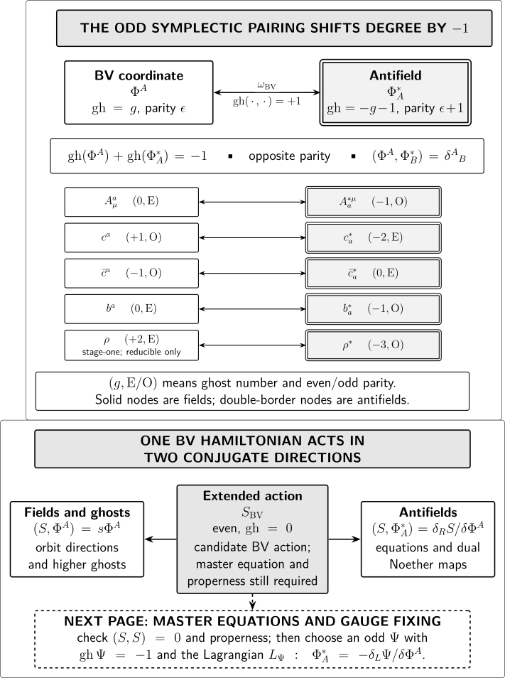
The shifted pairing sends $(g,\epsilon)$ to $(-g-1,\epsilon+1)$ and gives an antibracket of degree $+1$. The diagram is schematic and follows this page’s left/right-derivative convention. Its dashed lower band is a continuation: the classical master equation must still be checked, and $\Phi^*=-\delta_L\Psi/\delta\Phi$ selects a gauge-fixing Lagrangian only under the hypotheses developed on the next page.

A based Maxwell complex on a bounded region

Return to the smooth bounded connected spatial region $\Sigma$ and based redundancy group $\mathcal G_0$ of the BRST prerequisite. Work on a cylinder $I\times\Sigma$, with temporal endpoint data and the remaining boundary data chosen so that the Maxwell action is differentiable. Choose a finite, BRST-stable Galerkin core rather than an arbitrary mode cutoff: retain smooth Dirichlet scalar modes $e_\alpha$, their exact one-form gauge directions, compatible transverse gauge-field modes, and independent nonminimal spaces. Write

$$sA^r=R^r{}_\alpha c^\alpha, \qquad sc^\alpha=0, \qquad s\bar c^\alpha=b^\alpha, \qquad sb^\alpha=0.$$

Here $R^r{}_\alpha e_\alpha$ is the retained version of $\mathrm d e_\alpha$. The Dirichlet trace removes constant based parameters on connected $\Sigma$. Adjoin an algebraic shifted dual to every retained coordinate, so the finite odd form is

$$\begin{aligned} \omega_N={}& \boldsymbol\delta A_r^*\wedge\boldsymbol\delta A^r +\boldsymbol\delta c_\alpha^*\wedge\boldsymbol\delta c^\alpha\\ &+\boldsymbol\delta\bar c_\alpha^*\wedge\boldsymbol\delta\bar c^\alpha +\boldsymbol\delta b_\alpha^*\wedge\boldsymbol\delta b^\alpha. \end{aligned}$$

Let $S_{0,N}$ be a gauge-invariant Maxwell action on the retained modes, with $R^r{}_\alpha$ constant, and set

$$S_N = S_{0,N} +A_r^*R^r{}_\alpha c^\alpha -\bar c_\alpha^*b^\alpha.$$

The four coordinate checks are immediate:

$$\begin{aligned} (S_N,A^r)&=R^r{}_\alpha c^\alpha, & (S_N,c^\alpha)&=0,\\ (S_N,\bar c^\alpha)&=b^\alpha, & (S_N,b^\alpha)&=0. \end{aligned}$$

The conjugate checks expose the other half of the complex:

$$\begin{aligned} (S_N,A_r^*)&=\frac{\partial S_{0,N}}{\partial A^r},\\ (S_N,c_\alpha^*)&=A_r^*R^r{}_\alpha, \qquad (S_N,b_\alpha^*)=-\bar c_\alpha^*. \end{aligned}$$

Applying $X_{S_N}$ once more to $c_\alpha^*$ gives

$$X_{S_N}^2c_\alpha^* = \frac{\partial S_{0,N}}{\partial A^r} R^r{}_\alpha =0.$$

The last equality is precisely the finite Noether identity following from gauge invariance of $S_{0,N}$. This one chain displays the orbit generator, its dual Noether map, and the equations of motion without a formal continuum transpose or an integration by parts. It is also an exact controlled check of the degree and sign package.

The same model has three complementary readings:

reading	bounded-region meaning
Orbit	$c
Charge	Boundary-nontrivial transformations and possible surface charges are outside this bulk ghost complex and are not made exact by adding bulk antifields.
Gauge fixed	The nonminimal pair $(\bar c,b)$ is present, but a Coulomb gauge condition and the Lagrangian $\Phi^*=-\delta_L\Psi/\delta\Phi$ are still a separate choice.

For Coulomb gauge, $M_0=\Delta_D$ on $H^2(\Sigma)\cap H_0^1(\Sigma)$, and the positive spectral operator is $-\Delta_D$. Its Dirichlet gap controls the local gauge slice; it has nothing to do with nondegeneracy of $\omega_N$. A Dirichlet condition on $c$ also does not impose the same trace condition on $c^*$: the antifield belongs to the shifted dual of the ghost domain.

The orbit/charge distinction is developed for field-independent boundary transformations in Assanioussi et al. 2024, §§ 3.1–3.3, arXiv v2, pp. 13–16, Open PDF. If boundary fields are retained, the bulk BV data must be joined to compatible boundary BFV data; the naive closed-manifold master identity acquires a boundary contribution. The structure and the Maxwell/Yang–Mills examples are given in Cattaneo, Mnev, and Reshetikhin 2014, §§ 2.1, 3.1.1–3.1.3, 3.7, 5.1.1, and 5.2.1, arXiv v3, pp. 5–11, 22, 26–27, and 31–33, Open PDF. Their examples are first-order and Euclidean; only their graded and boundary structure is imported here.

Compact Yang–Mills extension

On the smooth Dirichlet ghost core used by the BRST prerequisite, products preserve the zero trace. With antifields placed in the corresponding shifted dual spaces, the continuum expression is

$$\begin{aligned} S_{\mathrm{ext}}=S_{\mathrm{YM}} +\int\mathrm d^d x\,\biggl[ &A^{*\mu}_a(D_\mu c)^a +\frac g2c_a^*f^{abc}c^bc^c\\ &-\bar c_a^*b^a \biggr]. \end{aligned}$$

The antibracket reads all derivatives as direct field/dual pairings; no boundary trace is transferred by an unannounced integration by parts. The limit $f^{abc}\to0$ recovers the Maxwell Hamiltonian. None of this proves a global gauge slice, removes Gribov copies, or turns boundary-nontrivial transformations into redundancies.

What follows from the odd geometry

The logical implications are deliberately one-way:

input	licensed conclusion	not licensed
complete shifted field/dual pairing on the declared domain	an odd nondegenerate form of ghost number $-1$	Faddeev–Popov or Hessian invertibility
closedness plus nondegeneracy	an antibracket satisfying shifted Jacobi	a measure, regulator, or BV Laplacian
$S$ even with ghost number $0$	$(S,\cdot)$ is an odd degree-$+1$ Hamiltonian vector field	$(S,S)=0$ or nilpotency
$(S,S)=0$ on a suitable domain	$X_S^2=0$ by shifted Jacobi	the quantum master equation or anomaly freedom
reducibility maps	higher ghosts and their antifields	open closure or a finite tower
a BRST-stable bulk boundary domain	a bulk complex for the declared redundancy subgroup	conservation or vanishing of boundary charges

Indeed, for even $S$ the Jacobi identity gives the exact handoff formula

$$X_S^2F = \frac12\bigl((S,S),F\bigr).$$

The converse can fail by central or domain effects, so the next page starts from the master equation itself. A current account of the formalism stresses that infinite-dimensional nondegeneracy, the field-theoretic BV Laplacian, effective regularization, and boundary data remain additional constructions, not automatic consequences of the finite-dimensional algebra Cattaneo, Mnev, and Schiavina 2025, §§ 2, 4.1, 4.4, and 4.6, arXiv v1, pp. 1–4 and 10–14, Open PDF.

Common pitfalls

Antifields are not antiparticles, complex conjugates, or antighosts. An antifield is the opposite-parity coordinate paired with a specified BV field. The antighost $\bar c$ is itself a field and therefore has its own distinct antifield $\bar c^*$.

Odd does not mean automatically nilpotent. The odd form defines the antibracket and Jacobi identity. Nilpotency of $(S,\cdot)$ additionally needs the master equation, up to the stated central and domain qualifications.

Reducible does not mean open. Reducibility is a relation among gauge generators and calls for ghosts-for-ghosts. Open closure is failure of the commutator algebra to close away from the equations of motion and calls for higher antifield terms.

A Faddeev–Popov zero mode does not by itself establish reducibility. It may come from a stabilizer or reducibility direction $R_A\epsilon=0$. After those directions are separated, a remaining zero mode has $R_A\epsilon\ne0$ tangent to the chosen gauge slice. Reducibility is a relation among generators before gauge fixing, possibly only on shell.

A BV pairing does not choose a gauge. The odd symplectic space contains both fields and antifields. Gauge fixing selects an admissible Lagrangian subspace; one does not integrate independently over every Darboux coordinate.

Bulk antifields do not erase a boundary charge. The ghost domain still decides which transformations are treated as redundancy. Boundary degrees of freedom require an enlarged boundary-compatible construction.

Check your understanding

These checks reinforce the construction and do not carry a score or completion status.

1. Recover every antifield degree. Use the shift rule to find the parity and ghost number of the antifields of $A,c,\bar c,b$.

Solution

Opposite parity and ghost number $-1-g$ give

$$\begin{array}{c|cccc} \text{antifield}&A^*&c^*&\bar c^*&b^*\\ \hline \text{parity}&\text{odd}&\text{even}&\text{even}&\text{odd}\\ \operatorname{gh}&-1&-2&0&-1 \end{array}$$

The result also shows why $\bar c$ and $A^*$, despite both having ghost number $-1$, are different objects.

2. Test shifted antisymmetry on an even functional. Set $F=G=S$ with $\epsilon_S=0$ in the graded antisymmetry relation. What does it say about $(S,S)$?

Solution

The exponent is $(0+1)(0+1)=1$, so

$$(S,S)=-(-1)(S,S)=+(S,S).$$

This is an identity, not a vanishing condition. The classical master equation therefore contains information.

3. Check the Zinn-source sign. The preceding page contains $L^asc^a$. Compare it with the BV term $-c_a^*sc^a$.

Solution

Equality of the two terms requires

$$c_a^*=-L^a.$$

For the even gauge field the comparison is $A^{*\mu}_asA_\mu^a=K^{a\mu}sA_\mu^a$, so $A^{*\mu}_a=K^{a\mu}$ in the corresponding shifted chart. These signs provide an independent round trip to the Slavnov functional.

4. Separate reducibility from closure. For $\delta B=\mathrm d\Lambda$, identify the reducibility map and the required higher ghost.

Solution

The map is $Z:\lambda\mapsto\mathrm d\lambda$. Since $RZ\lambda=\mathrm d^2\lambda=0$, the one-form ghost has a scalar ghost-for-ghost of ghost number $2$. No equation of motion was used, so this example is off-shell reducible rather than open.

Where the construction continues

Master Equations and BV Gauge Fixing imposes the classical and quantum master equations, derives the gauge-fermion Lagrangian, and separates formal BV Laplacians from regulated quantum identities. The BV Complex and the Classical Master Equation develops the theorem-level homological construction. Shifted Symplectic, Poisson, and BV Geometry develops the derived geometric interpretation. For boundary fields, charges, and gluing, continue to Boundary Symmetry, Surface Charges, and Edge Modes and the BV–BFV treatment cited above.

References

• Assanioussi, Mehdi, Jerzy Kowalski-Glikman, Ilkka Mäkinen, and Ludovic Varrin. “On the Covariant Formulation of Gauge Theories with Boundaries.” Classical and Quantum Gravity 41, no. 11 (2024): 115007. DOI. Open PDF, arXiv v2.
• Batalin, I. A., and G. A. Vilkovisky. “Gauge Algebra and Quantization.” Physics Letters B 102, no. 1 (1981): 27–31. DOI.
• Batalin, I. A., and G. A. Vilkovisky. “Quantization of Gauge Theories with Linearly Dependent Generators.” Physical Review D 28, no. 10 (1983): 2567–2582. DOI. See the 1984 erratum below.
• Batalin, I. A., and G. A. Vilkovisky. “Erratum: Quantization of Gauge Theories with Linearly Dependent Generators.” Physical Review D 30, no. 2 (1984): 508. DOI.
• Cattaneo, Alberto S., Pavel Mnev, and Nicolai Reshetikhin. “Classical BV Theories on Manifolds with Boundary.” Communications in Mathematical Physics 332, no. 2 (2014): 535–603. DOI. Open PDF, arXiv v3.
• Cattaneo, Alberto S., Pavel Mnev, and Michele Schiavina. “BV Quantization.” In Encyclopedia of Mathematical Physics, 2nd ed., edited by Richard J. Szabo and Martin Bojowald, vol. 5, 543–555. Oxford: Elsevier, 2025. DOI. Open PDF, arXiv v1.
• Fuster, Andrea, Marc Henneaux, and Axel Maas. “BRST-Antifield Quantization: A Short Review.” International Journal of Geometric Methods in Modern Physics 2, no. 5 (2005): 939–964. DOI. Open PDF, arXiv v2.
• Gomis, Joaquim, Jordi París, and Stuart Samuel. “Antibracket, Antifields and Gauge-Theory Quantization.” Physics Reports 259, nos. 1–2 (1995): 1–145. DOI. Open PDF, arXiv v1.
• Schwarz, Albert. “Geometry of Batalin–Vilkovisky Quantization.” Communications in Mathematical Physics 155, no. 2 (1993): 249–260. DOI. Open PDF, arXiv v1.
• Zinn-Justin, Jean. Quantum Field Theory and Critical Phenomena. 5th ed. Oxford: Oxford University Press, 2021. DOI.