The BRST Differential and Gauge-Fixed Complex

The BRST differential turns the declared infinitesimal gauge redundancy into an odd differential on a ghost-number-graded algebra. For Yang–Mills theory with irreducible generators and an algebra that closes off shell, its action on $A,c,\bar c,b$ satisfies $s^2=0$ without using field equations or an inverse Faddeev–Popov operator. A Grassmann-odd gauge-fixing functional then produces the auxiliary-field, gauge-fixing, and ghost terms as one $s$ -exact deformation.

This is an algebraic construction inside a declared field and boundary domain. Using it as a gauge-fixed path integral additionally requires a regular local Faddeev–Popov patch; promoting it to a quantum identity requires compatible measure and regulator data and control of anomalies. Nilpotency alone neither chooses a global representative nor turns a charged boundary symmetry into a redundancy.

Required background. Ghosts, Auxiliary Fields, and Gauge-Parameter Dependence supplies $M_A$ , the independent ghost fields, the $b$ field, and the action signs used below. Lie Groups, Lie Algebras, and Exponential and Adjoint Maps supplies the adjoint bracket and Jacobi identity.

Helpful background. Chains, Homology, Cohomology, and Exact Sequences supplies the vocabulary of nilpotent complexes.

An odd differential for the Yang–Mills gauge algebra

Take Hermitian generators with $[T^a,T^b]=if^{abc}T^c$ , write $A_\mu=A_\mu^aT^a$ , and use

D_\mu=\partial_\mu-ig[A_\mu,\mathord\cdot], \qquad \delta_\epsilon A_\mu^a=(D_\mu\epsilon)^a.

Assume that the gauge transformations close without using the field equations and that, after declared stabilizers have been treated, their generators are irreducible. The algebra $\mathscr A$ generated by $A,c,\bar c,b$ and their derivatives is graded by Grassmann parity $|X|$ and ghost number. The BRST differential is a left-acting odd derivation

s:\mathscr A^n\longrightarrow\mathscr A^{n+1}, \qquad s(XY)=(sX)Y+(-1)^{|X|}X(sY),

which commutes with spacetime derivatives. On the four generators it is defined by

field	parity	ghost number	BRST variation
$A_\mu^a$	even	$0$	$sA_\mu^a=(D_\mu c)^a=\partial_\mu c^a+g f^{abc}A_\mu^bc^c$
$c^a$	odd	$+1$	$sc^a=-\dfrac g2 f^{abc}c^bc^c$
$\bar c^a$	odd	$-1$	$s\bar c^a=b^a$
$b^a$	even	$0$	$sb^a=0$

Thus $sA$ is the infinitesimal gauge displacement with the even parameter $\epsilon$ replaced by the odd ghost $c$ . The quadratic rule for $sc$ is not optional: it records the non-Abelian closure of two gauge displacements. The pair $(\bar c,b)$ is the nonminimal doublet that implements gauge fixing while preserving off-shell closure. These rules, their ghost numbers, and the gauge-fixed Yang–Mills action are developed in Srednicki 2007, § 74, pp. 448–451, eqs. (74.3)–(74.24), with the official first-printing corrections to eqs. (74.1) and (74.8) understood.

In matrix notation the ghost rule is

sc=igc^2.

Although each coefficient $c^a$ is odd, $c^2$ need not vanish: the coefficients anticommute while the generators do not. An unqualified formula such as $sc=-\tfrac12[c,c]$ is therefore avoided unless the combined Lie and Grassmann bracket has first been defined. A structural treatment of the graded differential appears in Barnich, Brandt, and Henneaux 2000, §§ 2.2–2.3, arXiv v3, pp. 7–9, eqs. (2.12)–(2.18), Open PDF.

The original formulations used different auxiliary-field conventions. In the 1975 BRS presentation without an independent $b$ , the second antighost variation closes only after the ghost equation of motion is used; the modern four-field form above makes that distinction visible Becchi, Rouet, and Stora 1975, § 2.A, pp. 4–7, eqs. (1)–(15), Open PDF. Tyutin’s independent formulation gives the odd transformation, invariant action, and unit Jacobian in Tyutin 1975/2008, Appendix F, pp. 21–22, eqs. (F.8)–(F.12), Open PDF.

Nilpotency follows from closure and the Jacobi identity

The nilpotency check is short, but its signs carry the content. For the ghost, the left Leibniz rule and associativity give

\begin{aligned} s^2c &=ig\,s(c^2) \\ &=ig\bigl[(sc)c-c(sc)\bigr] \\ &=-g^2\bigl(c^2c-cc^2\bigr)=0. \end{aligned}

In components, the coefficient of $c^bc^cc^d$ is the Jacobi identity for $f^{abc}$ . For the gauge field, first note that

\begin{aligned} s(D_\mu c) &=D_\mu(sc) -ig\bigl[(sA_\mu)c+c(sA_\mu)\bigr], \\ D_\mu(c^2) &=(D_\mu c)c+c(D_\mu c). \end{aligned}

Substituting $sc=igc^2$ and $sA_\mu=D_\mu c$ then gives

\begin{aligned} s^2A_\mu &=igD_\mu(c^2) -ig\bigl[(D_\mu c)c+c(D_\mu c)\bigr] \\ &=0. \end{aligned}

Finally,

s^2\bar c=sb=0, \qquad s^2b=0.

Because $s^2$ vanishes on every generator, it vanishes on all of $\mathscr A$ . No field equation, ghost propagator, or inverse $M_A^{-1}$ has entered. Closure and the Jacobi identity, together with retention of $b$ , give the displayed off-shell nilpotency. Irreducibility has a different role: it ensures that no further ghost levels are needed.

The figure collects the resulting arrows. Compare its solid BRST arrows with the separately styled local-slice, quantum, and BV limits; those bands are not additional actions of $s$ .

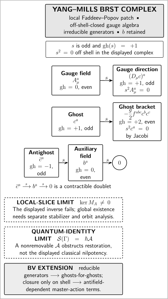
In a local irreducible Yang–Mills patch with off-shell closure, the ghost-number-one differential maps the gauge field to a ghost-valued gauge direction, the ghost to its quadratic Lie bracket, and the antighost to the auxiliary field and then zero; Faddeev–Popov zero modes, anomalies, and BV extensions are separate limits. — The solid arrows form the classical Yang–Mills BRST complex on a local Faddeev–Popov patch, with irreducible generators, off-shell closure, and $b$ retained. The dashed bands mark limitations rather than differential arrows: a zero mode can obstruct the local slice, and a nonremovable anomaly can obstruct the quantum identity without changing the displayed classical nilpotency. The BV band records the required extensions for reducible or on-shell-closing algebras. The diagram is schematic and not to scale.

Open the BRST complex as a full-size vector figure.

Text equivalent. In a local Faddeev–Popov patch with an irreducible off-shell-closed Yang–Mills algebra, $s$ is odd, raises ghost number by one, and squares to zero off shell when $b$ is retained. It maps the even field $A_\mu^a$ of ghost number zero to the odd expression $(D_\mu c)^a$ of ghost number one. It maps the odd ghost $c^a$ of ghost number one to the even ghost-number-two expression $-\tfrac g2f^{abc}c^bc^c$ ; the second applications vanish by closure and Jacobi. The odd antighost $\bar c^a$ of ghost number $-1$ maps to the even auxiliary field $b^a$ of ghost number zero, which maps to zero, so $(\bar c,b)$ is a contractible nonminimal doublet.

The figure also marks three distinct boundaries of that statement. A nonzero $\ker M_A$ makes the displayed local inverse fail and requires separate stabilizer and orbit analysis. A nonremovable breaking $\mathcal S(\Gamma)=\hbar\mathcal A+\cdots$ obstructs the quantum identity, not the classical calculation $s^2=0$ . Reducible generators require ghosts-for-ghosts, while closure only on shell requires antifield-dependent master-action terms.

Gauge fixing is generated by an odd functional

Let $F^a[A]$ be a bosonic gauge condition and define the site-convention Faddeev–Popov operator by

(M_A\epsilon)^a=\delta_\epsilon F^a[A].

For constant even $\xi$ , choose the gauge-fixing fermion

\Psi_F = \int d^dx\, \bar c^a\left(F^a[A]+\frac{\xi}{2}b^a\right).

The name means that $\Psi_F$ is Grassmann odd; it is a functional, not a new propagating fermion. Its ghost number is $-1$ , so $s\Psi_F$ is even and has ghost number zero. Because $\bar c$ is odd and $s$ acts from the left,

\begin{aligned} s\Psi_F &= \int d^dx\, \left[ b^a\left(F^a+\frac{\xi}{2}b^a\right) -\bar c^a\left(sF^a+\frac{\xi}{2}sb^a\right) \right] \\ &= \int d^dx\, \left( b^aF^a+\frac{\xi}{2}b^ab^a -\bar c^aM_A^{ab}c^b \right). \end{aligned}

The minus sign in the ghost term is exactly the graded Leibniz sign. This is the auxiliary-field convention established on the preceding page. The nonminimal pair and the gauge-fermion construction are given in Fuster, Henneaux, and Maas 2005, § 6, arXiv v2, pp. 13–15, eqs. (6.1)–(6.12), Open PDF.

For the gauge-invariant Yang–Mills action, set

S_{\Psi}=S_{\mathrm{YM}}+s\Psi_F.

On a domain preserved by $s$ ,

sS_{\Psi}=sS_{\mathrm{YM}}+s^2\Psi_F=0.

This is a classical off-shell statement. It also shows the useful exact relation

\frac{\partial S_{\Psi}}{\partial\xi} = s\left( \frac12\int d^dx\,\bar c^ab^a \right).

Turning that relation into gauge-parameter independence of a quantum expectation value requires more than the algebra; the required measure and anomaly qualifications are stated below.

Eliminating b changes closure on the antighost

For $\xi\neq0$ , the $b$ equation is $F^a+\xi b^a=0$ . Completing the square,

b^aF^a+\frac{\xi}{2}b^ab^a = \frac{\xi}{2} \left(b^a+\frac{F^a}{\xi}\right)^2 -\frac{F^aF^a}{2\xi},

gives the reduced action

S_{\mathrm{red}} = S_{\mathrm{YM}} +\int d^dx\, \left( -\frac{F^aF^a}{2\xi} -\bar c^aM_A^{ab}c^b \right).

The induced reduced transformation has

s_{\mathrm{red}}\bar c^a=-\frac{F^a}{\xi},

while the $A$ and $c$ rules are unchanged. Consequently,

s_{\mathrm{red}}^2\bar c^a = -\frac1\xi(M_Ac)^a \simeq0,

where $\simeq$ uses precisely the antighost equation $\delta S_{\mathrm{red}}/\delta\bar c^a=-(M_Ac)^a=0$ . Thus only closure in the antighost sector has become on shell; $s^2A=s^2c=0$ remains off shell in this Yang–Mills example. The reduced action itself is still invariant off shell: the variation of $-F^2/(2\xi)$ cancels the variation of $-\bar cM_Ac$ , and $s_{\mathrm{red}}(M_Ac)=s_{\mathrm{red}}^2F=0$ . This distinction is analyzed in Fuster, Henneaux, and Maas 2005, § 7, arXiv v2, p. 17, eqs. (7.5)–(7.10), Open PDF.

At $\xi=0$ , $b$ is a Lagrange multiplier imposing $F=0$ and cannot be eliminated by division by $\xi$ .

A based Coulomb complex on a bounded region

The boundary decides which gauge directions the ghost represents. Work at each time on a smooth, bounded, connected spatial domain $\Sigma$ , with a trivial bundle and compact structure group $K$ . Let $\iota:\partial\Sigma \hookrightarrow\Sigma$ and impose zero tangential pullback $\iota^*A=0$ . Declare as redundancy only the based group

\mathcal G_0 = \left\{ g:\Sigma\to K \ \middle|\ g|_{\partial\Sigma}=1 \right\}.

Its infinitesimal parameters, and hence the ghost, have zero boundary trace. Choose Coulomb gauge

F[A]=\partial_iA_i, \qquad M_A=\partial_iD_i.

The sign is the convention used throughout this chapter; the positive spectral operator on a Coulomb slice is $\mathcal M_A=-M_A$ .

Here is one BRST-stable continuum realization. Let $n=\dim\Sigma$ and choose $k>n/2+1$ . With $Y=L^2(\Sigma,\mathfrak k)$ ,

\begin{aligned} A&\in H^k(\Sigma,T^*\Sigma\otimes\mathfrak k), &\qquad \iota^*A&=0, \\ \operatorname{Dom}(M_A) &=H^2(\Sigma,\mathfrak k)\cap H_0^1(\Sigma,\mathfrak k), & M_A&:\operatorname{Dom}(M_A)\to Y, \\ \bar c,b&\in Y. && \end{aligned}

For the classical nonlinear algebra, take $c$ in the smooth Dirichlet core of $M_A$ , or in $H^{k+1}\cap H_0^1$ . Any later regulator or completion must be shown to preserve both the differential and the boundary domain. Use the invariant $L^2$ pairing to regard $\bar c$ as the odd dual variable to the codomain of $M_A$ and $b$ as its even partner. This choice makes every BRST map stay inside the declared space:

$\iota^*(sA)=\iota^*(Dc)=0$ because the trace of $c$ is zero;
$sc=-\tfrac g2f^{abc}c^bc^c$ again has zero trace; and
$s\bar c=b$ , $sb=0$ preserve the two copies of $Y$ .

The Coulomb gauge-fixing fermion and its variation are therefore

\Psi_C = \int dt\, \left\langle \bar c,\partial_iA_i+\frac{\xi}{2}b \right\rangle_Y,

\begin{aligned} s\Psi_C = \int dt\, \biggl[ &\left\langle b,\partial_iA_i\right\rangle_Y +\frac{\xi}{2}\langle b,b\rangle_Y \\ &-\left\langle\bar c,\partial_iD_ic\right\rangle_Y \biggr]. \end{aligned}

No integration by parts has been used, so no unannounced boundary condition on $\bar c$ is needed. If one instead imposes Dirichlet traces on both $\bar c$ and $b$ , those conditions are BRST-stable before elimination, but eliminating $b$ also requires $F[A]$ to lie in that Dirichlet domain; that is not automatic. Concrete Euclidean Maxwell boundary sets in which the gauge field, $c,\bar c,b$ , and the $b$ equation are all compatible are constructed in Moss and Silva 1997, § III, pp. 7–8, eqs. (30), (31), (33), and (37)–(38), Open PDF. More generally, the ghost boundary condition must be induced by the admitted gauge-parameter domain Vassilevich 2003, § 3.4, arXiv v3, pp. 27–29, eqs. (3.54)–(3.58), Open PDF.

The construction has three complementary readings:

reading	bounded-region meaning
Orbit	$sA=Dc$ is the odd tangent only to the based $\mathcal G_0$ orbit.
Charge	Boundary-nontrivial transformations are outside the ghost domain and may remain physical symmetries with surface charges.
Gauge fixed	$(\bar c,b)$ lives in the gauge-condition codomain and implements $F[A]$ together with the local Faddeev–Popov Jacobian.

The charge statement depends on the boundary phase-space setup; it is not a claim that every boundary transformation is charged. The distinction between redundancy and possible boundary symmetry is developed in Assanioussi, Kowalski-Glikman, Mäkinen, and Varrin 2024, §§ 3.1–3.3, arXiv v2, pp. 13–16, Open PDF.

Maxwell check

In the Abelian limit $f^{abc}\to0$ ,

sA_i=\partial_i c, \qquad sc=0, \qquad s\bar c=b, \qquad sb=0,

and $M_0=\Delta_D$ is the Dirichlet Laplacian in the site convention. If a Lie-algebra-valued parameter $\epsilon$ obeys $\Delta_D\epsilon=0$ and $\epsilon|_{\partial\Sigma}=0$ , then

0 = -\langle\epsilon,\Delta_D\epsilon\rangle_Y = \int_\Sigma d^nx\,|\nabla\epsilon|^2.

Connectedness gives $\epsilon=0$ . Thus there is no residual based Maxwell direction in this Dirichlet Coulomb problem. The ghosts are free and their determinant is field independent, although the $(\bar c,b)$ doublet remains part of the gauge-fixed complex.

For compact Yang–Mills theory, $sc$ is quadratic and $M_A=\partial_iD_i$ depends on $A$ , producing the ghost–gluon interaction. On a regular local patch near the vacuum, the Dirichlet gap makes $M_A$ invertible and the same gauge-fixed complex applies. If an even parameter $\epsilon\neq0$ obeys $M_A\epsilon=0$ , the ghost operator has the corresponding zero mode. With the based boundary condition, a covariantly constant parameter that vanishes on the boundary is zero; hence $D_A\epsilon\neq0$ , and the mode is a non-stabilizer orbit direction tangent to the gauge slice. It still need not produce a second finite copy. Those local-versus-global implications belong to Gribov Copies and the Limits of Local Gauge Fixing Vandersickel and Zwanziger 2012, §§ 2.1.5 and 2.2.1, arXiv v2, pp. 18 and 24–25, Open PDF.

The key separation is now explicit: invertibility of $M_A$ is needed for the local Faddeev–Popov slice and ghost propagator, but not for the algebraic calculation $s^2=0$ .

Classical exactness is not yet a quantum identity

For an even insertion $\mathcal O$ with $s\mathcal O=0$ , the formal gauge-parameter argument would use

0 \stackrel{?}{=} \int_{\mathcal C}\mathcal D\Phi\, s\left( \mathcal O\, \frac12\int d^dx\,\bar c^ab^a\, e^{iS_{\Psi}} \right).

The question mark matters. To replace it by an equality, one must establish all of the following:

the regulated measure, integration contour $\mathcal C$ , action, and boundary-condition domain are preserved by $s$ ;
integration by parts in field space produces no boundary contribution;
stabilizers and zero modes have been treated and the calculation remains in a valid local gauge-fixing patch;
the insertion is genuinely $s$ -closed in the declared complex; and
the regulator and renormalization prescription introduce no nonremovable BRST breaking.

These are quantum and analytic hypotheses, not consequences of the classical Leibniz rule. The measure and gauge-fermion qualifications are developed in Fuster, Henneaux, and Maas 2005, §§ 8–9, arXiv v2, pp. 19–22, Open PDF.

Schematically, a quantum breaking can appear as

\mathcal S(\Gamma) = \hbar\mathcal A+O(\hbar^2).

Consistency makes a local ghost-number-one BRST class a candidate anomaly. An exact breaking can be removed by an allowed local counterterm; a nontrivial class is an obstruction only after the regulator, locality, and counterterm problem have been specified. Classical $s^2=0$ remains true in either case Barnich, Brandt, and Henneaux 2000, § 2.6 and § 12.3, arXiv v3, pp. 16 and 119–121, eqs. (2.36)–(2.38), Open PDF.

The three tests should not be collapsed:

test	question	failure means
Local slice	Is $M_A$ invertible on the declared domain?	The local Faddeev–Popov coordinate or ghost inverse fails.
Classical algebra	Does the declared $s$ obey $s^2=0$ and preserve the field domain?	The four-field BRST complex is not defined as claimed.
Quantum identity	Do the regulated measure, action, contour, and counterterms preserve BRST?	The Ward or Slavnov identity needs restoration or is anomalous.

Where the four-field complex stops

The four transformations on this page are complete only for an irreducible algebra that closes off shell. If generators obey nontrivial relations among themselves, reducibility requires ghosts-for-ghosts. If their commutator closes only modulo equations of motion, antifield-dependent terms are needed to organize nilpotency. BV Fields, Antifields, and the Odd Symplectic Structure begins that extension; this page does not import its antibracket or master equation.

Nor has this page identified physical observables. BRST Cohomology and Physical Observables next declares the relevant functional or state complex and asks when closed representatives modulo exact ones have a physical interpretation. Slavnov–Taylor and Zinn-Justin Identities develops the renormalized functional identity only after the classical differential is in place.

Common pitfalls

Assuming that odd implies nilpotent. Parity alone gives the graded Leibniz sign. The quadratic rule for $sc$ and the Jacobi identity are what make $s^2A=s^2c=0$ .

Eliminating $b$ while retaining an unqualified off-shell claim. For $\xi\neq0$ , eliminating $b$ makes $s^2\bar c=0$ hold only with the antighost equation of motion. The $A$ and $c$ sectors remain off-shell nilpotent, and at $\xi=0$ this elimination is unavailable.

Treating a zero mode as failure of the BRST algebra. A zero mode of $M_A$ limits the local gauge slice. It neither spoils the Jacobi calculation nor, by itself, proves a separated finite Gribov copy.

Ghosting every boundary transformation. The ghost represents only the declared redundancy group. A boundary-nontrivial transformation that may carry a charge is outside the based ghost domain.

Reading $s\Psi$ as a quantum theorem. Classical exactness does not prove invariance of the regulated measure, contour, boundary domain, or renormalization prescription, and it does not exclude an anomaly.

Check your understanding

Starting from the left Leibniz rule, recover the sign of the ghost term in $s\Psi_F$ .

Check

Since $|\bar c|=1$ , $s[\bar c(F+\xi b/2)]=b(F+\xi b/2)-\bar c(sF+\xi sb/2)$ . Using $sF=M_Ac$ and $sb=0$ gives $-\bar cM_Ac$ .
Take the Abelian limit of the nilpotency calculation.

Check

When $f^{abc}=0$ , $sc=0$ and $D_\mu c=\partial_\mu c$ . Hence $s^2A_\mu=\partial_\mu(sc)=0$ , while the nonminimal pair still obeys $s\bar c=b$ and $sb=0$ .
For $\xi\neq0$ , identify exactly which closure statement changes after eliminating $b$ .

Check

The induced rule is $s_{\mathrm{red}}\bar c=-F/\xi$ , so $s_{\mathrm{red}}^2\bar c=-(M_Ac)/\xi$ vanishes with the antighost equation of motion. The $A$ and $c$ transformations are unchanged and remain off-shell nilpotent.
Distinguish a based zero mode from a charged boundary transformation.

Check

An even parameter $\epsilon\neq0$ with zero boundary trace and $M_A\epsilon=0$ is a residual tangent direction of the gauge slice; the ghost operator has the corresponding zero mode. A transformation with nonzero boundary value is outside $\mathcal G_0$ ; it is not represented by this ghost and may instead generate a boundary charge, depending on the phase-space boundary data.

References

Assanioussi, Mehdi, Jerzy Kowalski-Glikman, Ilkka Mäkinen, and Ludovic Varrin. “On the Covariant Formulation of Gauge Theories with Boundaries.” Classical and Quantum Gravity 41, no. 11 (2024): 115007. DOI. Open PDF, arXiv v2.
Barnich, Glenn, Friedemann Brandt, and Marc Henneaux. “Local BRST Cohomology in Gauge Theories.” Physics Reports 338, nos. 5–6 (2000): 439–569. DOI. Open PDF, arXiv v3.
Becchi, C., A. Rouet, and R. Stora. “Renormalization of Gauge Theories.” Les rencontres physiciens-mathématiciens de Strasbourg – RCP25 22 (1975), talk no. 10: 1–57. Institut de Recherche Mathématique Avancée – Université Louis Pasteur. Report 75/P.723. Stable record. Open PDF.
Fuster, Andrea, Marc Henneaux, and Axel Maas. “BRST-Antifield Quantization: A Short Review.” International Journal of Geometric Methods in Modern Physics 2, no. 5 (2005): 939–964. DOI. Open PDF, arXiv v2.
Moss, Ian G., and Pedro J. Silva. “BRST-Invariant Boundary Conditions for Gauge Theories.” Physical Review D 55, no. 2 (1997): 1072–1078. DOI. Open PDF.
Srednicki, Mark. Quantum Field Theory. Cambridge: Cambridge University Press, 2007. DOI. Author page and errata.
Tyutin, I. V. “Gauge Invariance in Field Theory and Statistical Physics in Operator Formalism.” P. N. Lebedev Physical Institute Preprint 39 (1975). English translation, arXiv:0812.0580v2 (2008). Stable record. Open PDF.
Vandersickel, Nele, and Daniel Zwanziger. “The Gribov Problem and QCD Dynamics.” Physics Reports 520, no. 4 (2012): 175–251. DOI. Open PDF, arXiv v2.
Vassilevich, D. V. “Heat Kernel Expansion: User’s Manual.” Physics Reports 388, nos. 5–6 (2003): 279–360. DOI. Open PDF, arXiv v3.