Gauging a Higher-Form Symmetry

Gauging a $p$-form symmetry promotes its prescribed $(p+1)$-form background to dynamical higher-gauge data, quotients by higher-gauge transformations, and sums or integrates over the allowed global sectors. That operation changes the theory: it projects unattached charged operators, permits new flux sectors, and, for an anomaly-free finite Abelian symmetry, produces a Pontryagin-dual symmetry of complementary degree.

The sum is meaningful only after the full background family, anomaly test, measure, topological weights, tangential structure, and boundary completion have been fixed. This page develops the finite Abelian construction for an ordinary invertible internal $A^{(p)}$ on a closed oriented $d$-manifold, with $0\leq p\leq d-2$, and contrasts it with continuous higher-form gauging. Non-Abelian or non-invertible defect gauging, full differential cohomology, and lattice implementation are later specializations.

Required background. Higher-Form Currents, Charges, Backgrounds, and Ward Identities supplies the $(p+1)$-form background, its gauge transformation, and the finite-versus-continuous distinction. Gauging Continuous and Finite Symmetries supplies the general gaugeability test, groupoid measure, projection, twisted sectors, and distinction between a fixed source and a dynamical field.

Helpful background. Characteristic Classes and Chern–Weil Theory supplies the language of global topological sectors and quantized weights.

Gauging promotes the higher background field

Let $A$ be a finite Abelian group and let $A^{(p)}$ be an exact, invertible $p$-form symmetry of a theory $\mathcal T$. On a chosen cellular or Čech model of $M$, a flat background is a cocycle

$$b\in Z^{p+1}(M;A), \qquad b\longmapsto b+\delta\lambda_p, \qquad \lambda_p\in C^p(M;A).$$

The charged objects have $p$-dimensional spacetime support, while the topological symmetry operators have dimension $d-p-1$ and codimension $p+1$. In the continuous Abelian description, the current convention is $j_{p+1}$ with closed dual $\widetilde j_{d-p-1}=\star j_{p+1}$, and the background has degree $p+1$. A finite symmetry keeps the same support and background degree but generally has no local Noether current.

The fixed-background functional $Z_{\mathcal T}[M;b]$ is a probe. Gauging does not mean selecting one value of $b$: it makes $b$ dynamical, identifies gauge-equivalent representatives, and includes every allowed cohomology class. Write

$$\widehat A=\operatorname{Hom}(A,U(1))$$

for the Pontryagin-dual group. A background for the prospective dual symmetry is

$$\widehat b\in H^{d-p-1}(M;\widehat A).$$

Inside cohomological brackets we identify $U(1)\cong\mathbb R/\mathbb Z$ additively. Thus $\langle\widehat b\smile b,[M]\rangle$ and $\langle\chi(b),D\rangle$ are $\mathbb R/\mathbb Z$-valued, and $\exp(2\pi i\,\cdot)$ returns the corresponding phase. Outside such brackets, $\chi(a)$ denotes that $U(1)$ phase directly.

In an untwisted or topologically weighted finite gauging, a useful closed-manifold convention is

$$\begin{aligned} Z_{\mathcal T/A^{(p)}}[M;\widehat b] ={}&\mu_{p,A}(M) \sum_{[b]\in H^{p+1}(M;A)} Z_{\mathcal T}[M;b]\,\Theta[b] \\ &\times \exp\!\left( 2\pi i\left\langle \widehat b\smile b,[M] \right\rangle \right). \end{aligned}$$

Here $\Theta[b]\in U(1)$ is a separately chosen, gauge-invariant local topological weight; $\Theta=1$ defines the untwisted example below. The evaluation pairing between $\widehat A$ and $A$ is implicit in the cup product. Its degrees add correctly,

$$(d-p-1)+(p+1)=d,$$

so the exponent can be evaluated on the oriented fundamental class $[M]$. Closedness and cochain Stokes show that changing either cocycle by a coboundary leaves the phase unchanged on closed $M$. Reversing the orientation of $M$ complex-conjugates it.

The factor $\mu_{p,A}(M)$ is not a universal $1/\lvert H^{p+1}(M;A)\rvert$. Gauge-for-gauge transformations themselves have automorphisms. In a standard finite homotopy-cardinality convention,

$$\mu_{p,A}(M) =\prod_{i=0}^{p} \left\lvert H^i(M;A)\right\rvert^{(-1)^{p+1-i}}.$$

Other normalizations can differ by declared local invertible factors, but a gluing-compatible measure must be specified. The higher-groupoid measure and its boundary-relative extension are derived in Monnier 2015, §§ 4–5, arXiv v3, pp. 6–7, eqs. (4.1)–(4.3) and (5.3), Open PDF, with Monnier’s gauge-field degree set to $p+1$ in the notation used here. The finite Fourier-transform form of the gauging and its conventional overall normalization appear in Gaiotto et al. 2015, § 6, arXiv v2, pp. 33–39, especially eqs. (6.1)–(6.2), Open PDF.

Continuous gauging is a different operation. A compact dynamical $(p+1)$-form connection $\mathcal B_{p+1}$ has curvature $H_{p+2}$ and requires a path-integral measure, gauge fixing or an equivalent quotient prescription, a regulator, and chosen kinetic or topological dynamics. If $p\leq d-3$ and magnetic defects are absent, such a field can support a magnetic $U(1)^{(d-p-3)}$ candidate. This continuous degree is not obtained by substituting $U(1)$ into the finite formula above.

Gaugeability and global choices come before the sum

The local fusion law of symmetry defects is necessary but not sufficient for gauging. The functional $Z_{\mathcal T}[M;b]$ must exist coherently for the complete allowed family of higher backgrounds, including nontrivial topology and the junctions that resolve a cocycle network. It must descend to gauge-equivalence classes after the selected counterterms and weights are included.

Before carrying out the sum, fix all of the following:

• the exact symmetry group and its faithful action on genuine operators;
• the allowed global background sectors and all gauge-for-gauge transformations;
• a gluing-compatible measure, including automorphism factors;
• the local kinetic terms or finite topological weight $\Theta[b]$;
• any spin, orientation, quadratic-refinement, or other tangential data;
• the treatment of singular defects, endpoints, and boundaries; and
• the operator spectrum against which projection and attachment are tested.

An uncancelled ‘t Hooft anomaly means that no counterterm makes the complete background functional gauge covariant in the required way. It obstructs standalone gauging in the same dimension unless extra degrees of freedom or inflow cancel it. A boundary similarly requires boundary conditions or boundary degrees of freedom that absorb the gauge variation; the closed-manifold formula cannot simply be copied unchanged.

The anomaly obstruction, promotion of a higher background, and finite dual symmetry are stated in Bhardwaj et al. 2024, § 4.3, arXiv v2, pp. 84–90, especially Statements 4.4–4.5, Open PDF.

Topological weights are theory data, not harmless normalization choices. For cyclic backgrounds, expressions colloquially written as a “$b\smile b$ term” can require a Pontryagin square, parity-dependent quantization, and spin or non-spin qualifications. Different allowed $\Theta$ define different gaugings and can change the genuine dyonic operators. These choices and their line-operator consequences are exhibited in Gaiotto et al. 2015, § 6, arXiv v2, pp. 34–39, Open PDF and Kapustin and Seiberg 2014, § 7, arXiv v2, pp. 27–31, especially pp. 28–30, Open PDF.

The process map below separates the prerequisite gate from the actual sector sum. Inspect the failed branch first: neither quotienting nor the dual-symmetry conclusion is licensed until the gaugeability and global-data checks pass.

For this map, let $K^{(p)}\subseteq G^{(p)}$ be the subgroup being gauged and let $H$ be the subgroup of its normalizer that preserves every gauging choice. Set $K=G=A$ for the full finite gauging above. The possible residual action is the faithful image of $H/K$, not a formal $G/K$ in general.

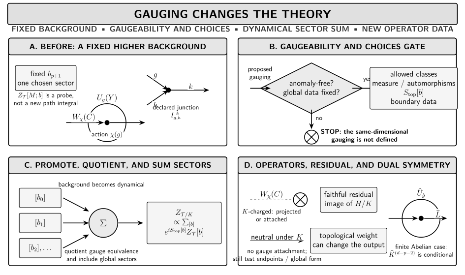
Gauging promotes a fixed $(p+1)$-form background to dynamical data only after the anomaly, sector, measure, topological-weight, tangential, and boundary choices pass. The output contains projected or attached operators and new sectors, together with a faithful residual image of $H/K$ when it exists; a finite Abelian gauging has a conditional $\widehat K^{(d-p-2)}$ dual symmetry. The diagram is schematic and not to scale; its line, loop, and junction icons encode operator relations rather than literal support dimensions.

Swipe horizontally to inspect the complete process, or open the vector figure at full size.

The table is the complete nonvisual reading of the process map.

What is fixed, summed, and changed by higher-form gauging

Datum	Before gauging	Gauging operation	After or qualification
Background	One prescribed higher connection or cocycle	Promote it and quotient its gauge hierarchy	It is dynamical rather than a source
Gaugeability	Full background functional and defect network	Test local, large, and junction gauge covariance	An uncancelled anomaly stops standalone gauging
Global sectors	Allowed topology and tangential data	Sum or integrate with automorphism weights	Measure, boundary data, and topological weight matter
Charged operator	Genuine operator in a nontrivial character	Average its higher-gauge orbit	Unattached version is projected; an attached version can remain
Neutral operator	Operator on which the gauged subgroup acts trivially	No higher-gauge attachment is required	Still test endpoints, screening, and global form
Linked action	A symmetry sheet measures a charged support by its character	Turn that sheet into gauge redundancy and average its label	The character average becomes the local projection test
Junction	Fusion incidence plus declared junction and coherence data	Sum only networks compatible with that data	The dual network needs its own junction data
Defect network	Fixed symmetry sheets and declared junctions	Sum compatible networks and rearrangements	Flux or twisted sectors become dynamical data
Residual symmetry	A larger symmetry may normalize the gauged subgroup	Retain only transformations preserving all gauging choices	The faithful image of H/K is conditional; G/K is not general
Dual symmetry	No dual action before the sum	Fourier-pair the new sectors	Finite Abelian case gives complementary-degree Pontryagin dual
Boundary	Boundary conditions and possible edge data	Choose relative sectors and cancel boundary variation	Closed-bulk formula alone is insufficient

Gauging changes operators and sectors

Let a genuine $p$-dimensional operator $W_\chi(C)$ transform in a character $\chi\in\widehat A$. Locally, averaging over a gauge transformation that links it gives the finite character projector

$$\frac{1}{\lvert A\rvert} \sum_{a\in A}\chi(a) =\delta_{\chi,1}.$$

Thus an unattached nonneutral insertion is projected from a gauge-invariant correlator. This does not mean that every charged operator vanishes or that dynamical screening has occurred. It means that the naked operator is no longer genuine after the old global transformation becomes gauge redundancy.

Suppose $C=\partial D$ for a $(p+1)$-chain $D$. Normalize the operator’s higher-gauge covariance as

$$W_\chi(C) \longmapsto \exp\!\left( 2\pi i\left\langle\chi(\lambda_p),C\right\rangle \right)W_\chi(C).$$

Then the $(p+1)$-chain-attached combination

$$W_\chi(C;D) =W_\chi(C) \exp\!\left( -2\pi i\left\langle\chi(b),D\right\rangle \right)$$

is gauge invariant: cochain Stokes converts the variation of the second factor into the inverse phase on $C=\partial D$. Replacing $D$ by another filling changes the insertion by the Wilson operator of $b$ on the closed cycle formed by the two fillings. The attachment is therefore physical data, not a disposable notation.

Neutral composites can survive without this attachment, subject to the ordinary endpoint, screening, and global-form tests. Conversely, defects that were twisted sectors of the original theory can become genuine operators after gauging and carry charge under the new dual symmetry. This exchange between charged and twisted sectors is developed in Bhardwaj et al. 2024, § 4.3, arXiv v2, pp. 90–94, Open PDF.

First application: gauge a finite cyclic electric one-form symmetry

Consider a four-dimensional compact $U(1)$ theory on a closed oriented Euclidean manifold $M$. Let $\mathfrak a$ be a faithfully normalized compact connection, $f=\mathrm d\mathfrak a$ locally, with

$$\frac{1}{2\pi}\int_{\Sigma_2}f\in\mathbb Z$$

for every closed oriented two-cycle $\Sigma_2$. Take $\theta=0$, keep magnetic backgrounds trivial, and include a complex scalar whose dynamical electric charges generate exactly $N\mathbb Z$, with $N\geq2$. Assume that the residual electric $\mathbb Z_N^{(1)}$ symmetry is exact and anomaly-free on this restricted background and that its invertible group-like surface network has coherent topological junctions.

Before gauging: line, surface, and junction

For a closed oriented line $C$, the Wilson operator and its unscreened charge are

$$W_n(C)=\exp\!\left(i n\oint_C\mathfrak a\right), \qquad r=[n]_N\in\mathbb Z_N.$$

Let $U_\alpha(\Sigma)$ be the symmetry surface labelled by $\alpha\in\mathbb Z_N$. For closed, oriented, disjoint $C$ and $\Sigma$ in a linking ball, with every other insertion $\mathcal X$ outside the sweep and the unlinked surface removable afterward, fix the positive unit-link convention by

$$\begin{aligned} \left\langle U_1(\Sigma)W_1(C)\mathcal X\right\rangle ={}&e^{2\pi i/N} \left\langle W_1(C)\mathcal X\right\rangle \\[-2pt] &\text{when }\operatorname{Lk}(\Sigma,C)=+1. \end{aligned}$$

The full character action is

$$\left\langle U_\alpha(\Sigma)W_n(C)\mathcal X\right\rangle = \exp\!\left( \frac{2\pi i}{N}\alpha r\operatorname{Lk}(\Sigma,C) \right) \left\langle W_n(C)\mathcal X\right\rangle.$$

Reversing either support orientation negates the linking number and inverts the phase. The surfaces fuse as

$$U_\alpha\otimes U_\beta \simeq U_{\alpha+\beta\;\mathrm{mod}\;N}.$$

For two incoming sheets and one outgoing sheet meeting along an oriented line $\ell$, declare a junction

$$I_{\alpha,\beta}^{\ \gamma}(\ell): U_\alpha\otimes U_\beta\longrightarrow U_\gamma, \qquad \alpha+\beta-\gamma=0\pmod N.$$

The character compatibility check is

$$\begin{aligned} \chi_r(\alpha)\chi_r(\beta)\chi_r(\gamma)^{-1} &=\exp\!\left[ \frac{2\pi i}{N}r(\alpha+\beta-\gamma) \right] \\ &=1. \end{aligned}$$

The congruence is necessary, but it neither constructs nor normalizes the junction and does not prove associativity or higher coherence. These compact-$U(1)$, linking, fusion, and charge-$N$ facts are bounded consequences of the global form, matter spectrum, and declared defect network; see Gaiotto et al. 2015, §§ 3 and 4.1, arXiv v2, pp. 11–18, especially eqs. (3.1)–(3.4), Open PDF.

The dynamical cocycle projects naked lines

Couple the electric symmetry to a flat two-cocycle

$$b\in Z^2(M;\mathbb Z_N), \qquad b\longmapsto b+\delta\lambda_1, \qquad \lambda_1\in C^1(M;\mathbb Z_N),$$

and gauge it by the untwisted, normalized sum over $[b]$. On a small link of the Wilson line, the gauge average is exactly

$$\frac{1}{N}\sum_{\alpha=0}^{N-1} \exp\!\left(\frac{2\pi i}{N}\alpha r\right) =\delta_{r,0}.$$

Only $r=0$ survives as an unattached Wilson line in the original normalization. A line with $r\neq0$ can instead be made gauge invariant by choosing an oriented two-chain $D$ with $\partial D=C$ and inserting

$$W_n(C;D) =W_n(C) \exp\!\left( -\frac{2\pi i}{N}r\left\langle b,D\right\rangle \right).$$

The second factor is the required dynamical surface attachment. This projection is distinct from matter screening: charge-$N$ matter already allows $W_N$ to end, whereas gauging makes every nonneutral residue class $r$ require a surface.

Indeed, if $P:y\to x$ and the charge-$N$ scalar is $\Phi_N$, then

$$\Phi_N^\dagger(x)\,W_N(P:y\to x)\,\Phi_N(y)$$

is gauge invariant. It exhibits a dynamical endpoint for $W_N$ independently of the new higher-gauge projection.

The output contains a dual network

Because $\widehat{\mathbb Z_N}\cong\mathbb Z_N$, the gauged theory has a dual one-form symmetry under the stated finite, Abelian, closed-bulk hypotheses. Its surface operator can be represented by

$$\left\langle m,x\right\rangle =\frac{mx}{N}\pmod 1, \qquad m,x\in\mathbb Z_N,$$

which fixes the standard self-duality pairing, and then by

$$\widehat U_m(\Sigma) =\exp\!\left( \frac{2\pi i}{N}m\left\langle b,\Sigma\right\rangle \right), \qquad m\in\mathbb Z_N.$$

The original $U_\alpha$ sheets have become part of the summed gauge redundancy rather than independent global-symmetry defects. The new dual surfaces instead measure the $b$-flux sectors created by the sum.

A $b$-flux disorder line $\widehat T_s(C')$ of charge $s\in\mathbb Z_N$ is defined by the oriented small-link condition

$$\left\langle b,S^2_{\mathrm{link}}\right\rangle=s\pmod N.$$

It is detected by the dual surface through the correlator identity

$$\begin{aligned} \left\langle \widehat U_m(\Sigma)\widehat T_s(C')\mathcal X \right\rangle ={}&\exp\!\left( \frac{2\pi i}{N}ms\operatorname{Lk}(\Sigma,C') \right) \\ &\times \left\langle\widehat T_s(C')\mathcal X\right\rangle. \end{aligned}$$

inside correlators with the same closed-support and removal hypotheses. The dual surfaces fuse additively. A declared two-in/one-out dual junction with labels $m_1,m_2,m_3$ obeys

$$m_1+m_2-m_3=0\pmod N,$$

again as an incidence check rather than a construction of junction data.

Gauging the electric subgroup changes the global form to $U(1)/\mathbb Z_N$. Although this quotient is abstractly isomorphic to $U(1)$, it is not the same normalization. Locally one may write

$$\mathfrak a'=N\mathfrak a, \qquad W_N(\mathfrak a)=W_1(\mathfrak a'),$$

so only $W_{N\ell}$ descends as an unattached Wilson line in the old normalization, while the quotient permits magnetic sectors fractional in the old flux unit. Charge, flux, bundle, and coupling data must all be translated. Nor should the new $\widehat{\mathbb Z_N}^{(1)}$ be assumed to split as an independent direct factor from a pre-existing magnetic symmetry. The compact-Abelian rescaling is explicit in Gaiotto et al. 2015, § 4.1, arXiv v2, p. 16, eq. (4.3), Open PDF. The more general quotient, attachment, and line-spectrum consequences are treated in Kapustin and Seiberg 2014, § 7, arXiv v2, pp. 27–31, Open PDF.

Nothing in this projection calculation decides whether the resulting theory confines, is gapless, or has a topological phase. Those are dynamical and state-dependent questions.

Residual and dual symmetries require hypotheses

Suppose a subgroup $K^{(p)}\subseteq G^{(p)}$ is gauged. Let $\mathcal D_{\mathrm{gauge}}$ denote the measure, topological weight, allowed sectors, tangential structure, and boundary data, and define

$$H=\left\{ g\in N_G(K):g\text{ preserves }\mathcal D_{\mathrm{gauge}} \right\}.$$

Because $K$ is normal in $H$, the candidate residual action is by $H/K$. The physical residual symmetry is its faithful image after quotienting any common kernel on the new genuine operator spectrum. Only when $K$ is normal in all of $G$ and every gauging choice is $G$-invariant does this reduce to a faithful form of $G/K$.

For finite Abelian $K$ and $p\leq d-2$, Fourier pairing of the new sectors produces

$$\widehat K^{(d-p-2)}.$$

Its charged objects have spacetime dimension $d-p-2$, while its topological symmetry operators have dimension $p+1$. Thus gauging a one-form symmetry in four dimensions again produces a one-form symmetry; gauging a zero-form finite Abelian symmetry in $d$ dimensions produces a $(d-2)$-form dual. Residual and dual factors can participate in an extension or mixed anomaly, so even $(H/K)\times\widehat K$ is not automatic.

For finite Abelian groups with $G$-invariant gauging data, the $G/K$ specialization, complementary dual degree, and possible mixed anomaly are summarized in Bhardwaj et al. 2024, § 4.3, arXiv v2, pp. 88–95, Open PDF.

With the untwisted finite Fourier kernel and compatible normalization, gauging the dual symmetry performs Fourier inversion. It returns the original theory only up to charge conjugation, a possible local invertible factor, and the translation of any chosen topological weight. This is a strong consistency check, not permission to ignore normalization or global sectors.

For a continuous compact higher gauge field, the magnetic candidate instead has degree $d-p-3$ when that degree is nonnegative and when no dynamical magnetic defects violate its conservation law. Non-Abelian zero-form gauging and non-invertible defect condensation require representation- or category-level data and are not governed by the finite character transform.

Method checks and failure modes

A proposed higher-form gauging should pass the following independent checks.

1. Degree check. The old background has degree $p+1$; a finite dual background has degree $d-p-1$; their cup product has degree $d$.
2. Gauge-variation check. Coboundary shifts leave every weight and the Fourier kernel invariant on the declared closed manifold, or their boundary variation is cancelled by explicit boundary data.
3. Measure check. Gauge automorphisms and gauge-for-gauge automorphisms are included. A sum over cohomology classes alone is not yet a complete path-integral normalization.
4. Operator check. Every original charged insertion is classified as neutral, projected, or equipped with a specified attachment; every new flux defect has a declared support and linking action.
5. Topology check. Nontrivial global sectors, torsion, tangential structure, and topological weights are part of the definition rather than optional afterthoughts.
6. Fourier check. When finite untwisted double gauging is claimed, the second sum recovers the original sector data with the declared normalization and charge-conjugation convention.

Stop the construction if the theory is known only at the trivial background, if an anomaly remains uncancelled, or if the measure and global sectors have not been specified. On a manifold with boundary, replace absolute cohomology by the appropriate relative or boundary-decorated data. For a continuous group, do not write a formal finite sum in place of the required functional measure, regulator, gauge fixing, and dynamics. For a non-normal subgroup or a nontrivial action on the gauging data, do not assert a residual quotient or a direct product with the dual symmetry.

Common pitfalls

Background coupling is not gauging. Evaluating $Z_{\mathcal T}[M;b_0]$ at one prescribed $b_0$ probes the symmetry. Gauging changes the theory by making $b$ dynamical and summing or integrating its gauge-equivalence classes.

An infinitesimal invariance test is not enough. Large transformations, nontrivial bundles or cocycles, junction moves, and boundaries can expose an obstruction invisible near the trivial background.

The sector sum is not uniformly averaged by fiat. Gauge and gauge-for-gauge automorphisms determine a gluing measure. A factor $1/\lvert H^{p+1}\rvert$ is not a universal replacement.

Charged operators do not all disappear. An unattached nonneutral operator is projected, while a higher-dimensional attached version may remain and old twisted defects may become genuine.

Projection is not screening. Projection follows from a new gauge redundancy. Screening asks whether actual dynamical endpoints identify a charge class; the predicates must be checked separately.

A finite dual formula is not a continuous one. Pontryagin duality gives the finite complementary degree. Continuous magnetic symmetry follows from a Bianchi identity for a chosen dynamical higher connection and has a different degree.

A topological weight is not decoration. Discrete theta data can change the genuine line or defect lattice. Spin and non-spin definitions can admit different weights.

Gauging does not choose a phase. Operator projection and new sectors are kinematic consequences of the operation. Confinement, spontaneous breaking, gaplessness, and topological order require separate dynamics.

Check your understanding

Use each checked answer to identify both the minimum calculation and the missing-data test.

1. In $d=5$, gauge a finite Abelian two-form symmetry. What is the degree of $b$, the degree of $\widehat b$, and the form degree of the dual symmetry?

Checked answer

Here $p=2$. The dynamical cocycle has degree $p+1=3$ and the dual background has degree $d-p-1=2$, so their cup product is a five-cocycle. The dual symmetry has form degree $d-p-2=1$. Its topological generators therefore have dimension $p+1=3$, while its charged defects are lines.

2. For a one-form symmetry $A^{(1)}$ on a closed connected manifold, what replaces a naive uniform sum over $H^2(M;A)$?

Checked answer

In the displayed homotopy-cardinality convention,

$$\mu_{1,A}(M) =\frac{\lvert H^0(M;A)\rvert} {\lvert H^1(M;A)\rvert}.$$

This factor multiplies the sum over $H^2(M;A)$. A boundary, a twist, or a different local invertible normalization requires a corresponding change; one should not silently replace the result by $1/\lvert H^2\rvert$.

3. In the $\mathbb Z_6^{(1)}$ example, evaluate the local projector for Wilson residues $r=4$ and $r=0$.

Checked answer

Character orthogonality gives

$$\frac{1}{6}\sum_{\alpha=0}^{5} e^{2\pi i\alpha r/6} =\delta_{r,0}.$$

The result is zero for $r=4$ and one for $r=0$. Thus the first naked line is projected and needs a dynamical two-surface attachment; the second passes this gauge-invariance test, though its screening and endpoint data still need to be checked.

4. Verify the sign in the attached operator under $b\mapsto b+\delta\lambda_p$.

Checked answer

For $\partial D=C$, cochain Stokes gives

$$\left\langle\chi(\delta\lambda_p),D\right\rangle =\left\langle\chi(\lambda_p),C\right\rangle.$$

The attachment with a minus sign therefore transforms by the inverse of the positive phase assigned to $W_\chi(C)$. Reversing the sign in either one convention requires reversing it in the other as well.

5. Why does $\alpha+\beta-\gamma=0\pmod N$ not prove that a surface junction exists, either before or after gauging?

Checked answer

The congruence verifies only label incidence and character compatibility for two incoming sheets and one outgoing sheet. Existence, normalization, junction-state dimension, associativity, and coherence are additional defect-network data. After gauging, compatible networks are summed, so omitting those data makes the gauged theory itself under-specified.

6. A compact continuous $(p+1)$-form connection is gauged in $d$ dimensions. May one immediately claim the finite dual $\widehat A^{(d-p-2)}$?

Checked answer

No. The finite statement follows from a finite Fourier transform. A continuous compact field instead has curvature degree $p+2$ and can have a magnetic $U(1)^{(d-p-3)}$ symmetry only if the degree is nonnegative and magnetic defects, boundaries, and anomalies do not spoil its Bianchi identity. Its measure, regulator, and dynamics must also be declared.

Continue to coupled backgrounds, topological models, and lattice realizations

Higher-Group Symmetry and Coupled Backgrounds explains when background transformations mix rather than factor. Higher-Group Operators, Gauging, and Anomalies then tests whether those coupled backgrounds can be gauged consistently.

BF Couplings and Discrete Topological Data constructs continuum finite-gauge realizations and their linking phases. Gauging, Equivariantization, Orbifolds, and Condensation develops the category-level operation when the finite character sum is no longer enough.

For regulated Hamiltonian realizations, continue to Lattice Gauge Theory and then Local Hilbert-Space Regulators, Quantum Links, and Finite Gauge Groups. Those treatments develop Gauss-law constraints and finite local Hilbert spaces beyond the analytical sector sum used here.

References

• Bhardwaj, Lakshya, Lea E. Bottini, Ludovic Fraser-Taliente, Liam Gladden, Dewi S. W. Gould, Arthur Platschorre, and Hannah Tillim. “Lectures on Generalized Symmetries.” Physics Reports 1051 (2024): 1–87. DOI. Open PDF, arXiv:2307.07547v2.
• Gaiotto, Davide, Anton Kapustin, Nathan Seiberg, and Brian Willett. “Generalized Global Symmetries.” Journal of High Energy Physics 2015, no. 2 (2015): 172. DOI. Open PDF, arXiv:1412.5148v2.
• Kapustin, Anton, and Nathan Seiberg. “Coupling a QFT to a TQFT and Duality.” Journal of High Energy Physics 2014, no. 4 (2014): 001. DOI. Open PDF, arXiv:1401.0740v2.
• Monnier, Samuel. “Higher Abelian Dijkgraaf–Witten Theory.” Letters in Mathematical Physics 105, no. 9 (2015): 1321–1331. DOI. Open PDF, arXiv:1502.04706v3.