Symmetry Realization and Breaking

Enter this chapter by the physical question, not by the word breaking. To decide whether a symmetry is spontaneously broken, begin with the exact physical symmetry, the selected state, and the order of the thermodynamic and source limits. To derive a Goldstone consequence, add the current, locality, spectral, spacetime, and dimensional hypotheses that turn broken realization into a statement about infrared modes. To interpret Higgs physics, first separate a physical global action from local gauge redundancy and then use gauge-invariant spectra and response.

The chapter develops ordinary global-symmetry realization, pure-phase selection, vacuum orbits, Goldstone existence and counting, nonlinear realizations, controlled explicit breaking, and the gauge-invariant Higgs distinction. It does not replace rigorous phase construction, numerical finite-size analysis, developed finite-density or spacetime-symmetry effective theory, chiral effective-theory matching, lattice gauge phase diagrams, or Higgs phenomenology. Those subjects have dedicated continuations below.

Helpful background. Vacua, States, and Representations supplies the distinction among a state, its observable algebra, and a Hilbert space representation. Clustering, Vacuum Assumptions, and Long-Range Correlations supplies the long-distance test used to distinguish a selected pure phase from a symmetric mixture. Neither is required merely to use this overview.

Parent volume. Symmetry and Gauge Structure

Jump to: choose a route · compare global and gauge realization · review the chapter

Diagnose your preparation

Use these observable checks instead of a score. An Unsure result identifies the shortest repair; it does not bar entry to the overview.

Theory symmetry and state symmetry. Ready: You can explain how an exact symmetry of the dynamics may fail to fix one state; enter Symmetry Realization and Order Parameters. Unsure: You would call every nonzero classical field a broken quantum symmetry. Repair: Use What Is a Symmetry of a QFT? and Vacua, States, and Representations.

Pure phases and clustering. Ready: You can say why a symmetric mixture may have a long-distance two-point plateau while failing clustering; enter Finite Volume, Thermodynamic Limits, and Pure Phases after the first page. Unsure: You regard a symmetric finite-volume ground state as proof that no broken phase exists. Repair: Use Clustering, Vacuum Assumptions, and Long-Range Correlations.

Actions, stabilizers, and quotients. Ready: Given a group action on a state, you can compute its stabilizer and distinguish the orbit $G/H$ from a quotient group acting on every object; enter Vacuum Orbits and Unbroken Subgroups. Unsure: You infer a particle count merely from the number of classical minima. Repair: Use Groups, Actions, Quotients, and Covers and Lie Groups, Lie Algebras, and Exponential and Adjoint Maps.

Currents, Ward identities, and poles. Ready: You can distinguish a renormalized conserved current from a formal classical expression and explain what a pole in a two-point function means; enter Goldstone’s Theorem after constructing the phase. Unsure: You infer a massless particle from a conserved-looking current without naming the state or spectral assumptions. Repair: Use Quantum Currents, Improvements, and Conservation and The Källén–Lehmann Representation.

Physical action versus gauge redundancy. Ready: You can name a gauge-invariant observable and explain why two configurations on one gauge orbit are not two physical vacua; enter Elitzur’s Theorem and the Gauge-Invariant Higgs Mechanism after the first page. Unsure: You treat a gauge-fixed scalar expectation value as a standalone physical order parameter. Repair: Use Gauge Fields, Redundancy, and Observable Content and The Free Maxwell Field and Gauge Redundancy.

Choose a route

Build a first coherent account. Read realization $\to$ limits $\to$ orbits $\to$ Goldstone theorem $\to$ counting $\to$ cosets $\to$ explicit breaking $\to$ gauge-invariant Higgs physics. At the end, you can keep phase selection, geometry, spectral consequences, low-energy coordinates, deformations, and gauge redundancy in their proper logical order.
Diagnose an ordered phase. Read realization $\to$ limits $\to$ orbits. At the end, you can classify the realization, construct a selected clustering phase, and identify one symmetry orbit and its stabilizer.
Test a Goldstone claim. Read realization $\to$ limits $\to$ theorem $\to$ counting and exceptions. Add the orbit page when $G/H$ supplies the proposed broken directions. At the end, you can separate existence of massless spectral weight from the regime-dependent count of independent modes.
Build a nonlinear low-energy description. Read realization $\to$ orbits $\to$ cosets. Add the theorem and counting pages to justify which modes propagate. At the end, you can construct the compensator, Maurer–Cartan components, and invariant local building blocks.
Follow controlled explicit breaking. Read realization $\to$ limits $\to$ theorem $\to$ pseudo-Goldstones. At the end, you can distinguish a temporary selector from a permanent deformation and derive the deformed Ward identity and angular mass matrix.
Translate Higgs language into physical statements. Read gauge redundancy $\to$ realization $\to$ Elitzur and invariant Higgs diagnostics. At the end, you can reject gauge-orbit degeneracy as physical vacuum degeneracy and replace a gauge-fixed scalar expectation value by invariant spectral and response questions.

The arrows are suggested reading order, not logical implication. The sidebar records a coherent full route, but a focused lookup need not traverse every earlier page. Each page’s background note states the actual dependencies.

From a theory symmetry to an infrared statement

Let an exact physical global group $G$ act on the observable algebra and on states. For a selected state $\omega$ , its preserved subgroup is

H_\omega = \left\{g\in G\mid g\mathbin{\cdot}\omega=\omega\right\}.

Spontaneous breaking means $H_\omega$ is a proper subgroup while the theory still has the exact symmetry $G$ . That definition already separates spontaneous breaking from a permanent symmetry-breaking interaction, an approximate relation, and an emergent symmetry valid only in a stated regime. It also explains why the state must be identified before an order parameter is interpreted.

For a noninvariant local observable $O$ and a source $J$ that selects an orientation $\theta$ , the standard phase construction has the order

\langle O\rangle_\theta = \lim_{J\to0^+} \lim_{\mathcal V\to\infty} \langle O\rangle_{\mathcal V,J,\theta}.

The volume family, boundary conditions, state preparation, and convergence of local observables must be specified, and clustering is then a check on the selected phase. If every finite-volume system has a unique symmetric state, removing $J$ before the volume limit instead returns the symmetric answer for a noninvariant $O$ ; the two procedures need not commute. The selector and finite-volume logic are developed in Tong 2019, §§ 2.1.1–2.1.2, pp. 50–58, Official PDF and Weinberg 1995, § 19.1, pp. 163–167.

Once a phase is selected, a smooth action of $G$ generates the orbit $G\mathbin{\cdot}\omega$ . When $G$ is a finite-dimensional Lie group and $H_\omega$ is closed,

G\mathbin{\cdot}\omega \simeq G/H_\omega, \qquad T_\omega(G\mathbin{\cdot}\omega) \simeq \mathfrak g/\mathfrak h_\omega.

This is the geometry of one orbit. It does not prove that the complete vacuum set is one orbit, nor does its dimension by itself count propagating particles. A Goldstone conclusion requires the additional current, locality, infinite-volume, translation, spectral, and—when using the relativistic spin-zero theorem—Lorentz assumptions. The regulated-current commutator and Ward identity then force massless spectral support rather than relying on an ill-defined global charge vector. In the Lorentz-invariant internal-symmetry setting, the independent modes match the broken directions; without Lorentz invariance, the charge-density matrix can pair broken generators into type-B modes. When the translation-invariant thermodynamic commutator-density limit exists with finite stable rank and the other internal-counting hypotheses hold, the relation

n_{\mathrm{NG}} = n_{\mathrm{br}} -\frac12\operatorname{rank}\rho

does not apply mechanically to broken spacetime generators. In local relativistic theories with sufficiently short-range interactions, infrared fluctuations obstruct the ordinary continuously broken phase in $1+1$ dimensions. The regime distinctions and hypotheses are summarized in Watanabe 2020, §§ 2.2, 2.6, and 3.2, pp. 3–10, Open PDF.

Relation	Input	Result	Guardrail
Defines	Exact physical group $G$ and selected state $\omega$	Preserved subgroup $H_\omega$	Breaking is a property of the state; explicit breaking changes the theory data
Requires an ordered limit	Finite-volume symmetric state plus temporary selector $J$	Selected infinite-volume clustering phase	A finite-volume vector or classical minimum does not establish the phase
Organizes	Selected vacuum and closed stabilizer $H$	Orbit $G/H$ and tangent $\mathfrak g/\mathfrak h$	One orbit need not be the full vacuum set, and tangent dimension is not yet a particle count
Implies under hypotheses	Broken current direction and the local Ward identity	Massless spectral support	Current existence, locality, state, spectrum, dimension, and spacetime symmetry must be checked
Refines	Broken directions	Type-A/type-B modes or redundant spacetime fluctuations	The valid count depends on charge densities and on independence of low-energy fields
Constructs	Local coordinates on $G/H$	Nonlinear transformations and invariant Maurer–Cartan building blocks	Geometry does not determine Wilson coefficients or prove the phase exists
Deforms	Permanent explicit breaker $\epsilon$	Current divergence, alignment, and possibly $m_{\mathrm{pG}}^2=O(\epsilon)$	The scaling requires a smooth restoring limit, a stable aligned vacuum, and a persistent light state
Contrasts	Global phase orbit versus local gauge orbit	Distinct physical vacua versus equivalent representatives	Gauge-fixed field expectations are not standalone physical phase diagnostics

Orbit dimension, the number of Goldstone modes, the number of disconnected vacua, and the number of gauge representatives are therefore four different quantities. Confusing any pair erases a required hypothesis or changes the physical question.

Global orbits and gauge orbits answer different questions

The figure makes the last row of the comparison concrete. Read the top panel as a sequence of physical state selections: an ordered limit can choose one of several globally related phases, and a Goldstone pole follows only after the theorem’s extra hypotheses are supplied. The bottom panel instead separates three levels: a local gauge transformation relates field and gauge potential representatives, gauge fixing may optionally choose one representative, and physical claims must be tested with gauge-invariant operators. The dashed boxes keep representative-level data distinct from physical diagnostics: the first displays two representatives of one orbit, and the second explicitly marks the gauge dependence of a gauge-fixed expectation. The solid final box marks the invariant diagnostics.

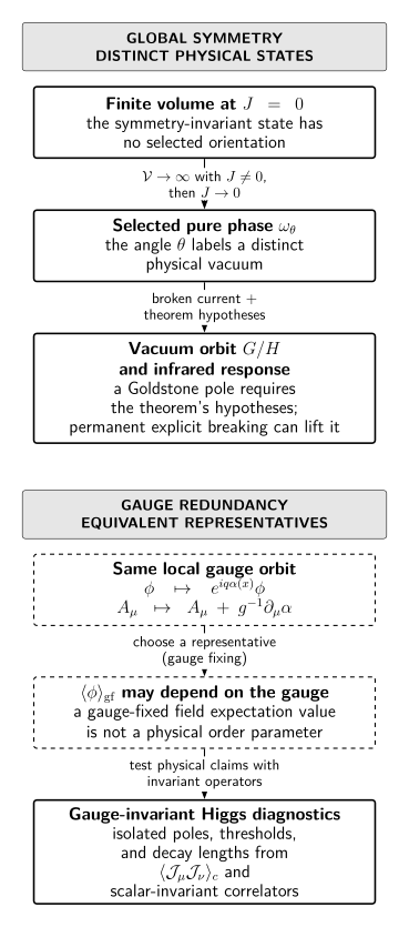
An ordered limit selects physically distinct vacua related by a global symmetry and yields a Goldstone pole only under theorem hypotheses; gauge transformations instead relate equivalent field and gauge-potential representatives, so Higgs claims require gauge-invariant correlators. — Global symmetry breaking and gauge-Higgs diagnostics follow different logical chains. In the upper chain, $\mathcal V\to\infty$ at nonzero selector $J$ followed by $J\to0$ can select a physical vacuum on $G/H$ ; a Goldstone pole is conditional on the current theorem’s hypotheses, and permanent explicit breaking can lift it. In the lower comparison, $(\phi,A_\mu)$ and $(e^{iq\alpha(x)}\phi,A_\mu+g^{-1}\partial_\mu\alpha)$ lie on one gauge orbit. Gauge fixing can choose a representative, but physical Higgs-like behavior is tested with connected gauge-invariant current and scalar correlators: isolated poles when they exist, and thresholds, decay lengths, or thermodynamic data more generally. The diagram is schematic and not to scale.

For compact, unfixed lattice gauge theories with a positive local Euclidean weight, Elitzur’s local-averaging argument gives a precise setting in which suitable bounded local gauge-variant expectations vanish; it does not turn every gauge-fixed remnant symmetry statement into a theorem about every continuum formulation. The physical conclusion is the narrower one used here: local transformations declared redundant do not connect distinct physical vacua. Gauge-invariant composite correlators, line operators, screening, thermodynamic singularities, and other invariant data carry the physical content. See Elitzur 1975, §§ I–IV, pp. 3978–3982 and Weinberg 1995, § 21.1, pp. 295–300.

Exact chapter guide

1. Symmetry Realization and Order Parameters

Start here to ask whether an exact physical symmetry of the theory fixes the selected state. The page distinguishes unbroken, spontaneous, explicit, approximate, and emergent realization; defines sufficient order-parameter tests; and explains why one vanishing candidate is inconclusive. After it, you can classify the theory data and state without using a classical minimum or a finite-volume vector as a substitute for phase selection. It uses What Is a Symmetry of a QFT? and Vacua, States, and Representations. Continue to the limits page for a robust phase construction or directly to the gauge-Higgs page when the central issue is redundancy.

2. Finite Volume, Thermodynamic Limits, and Pure Phases

This page asks why a symmetric finite-volume ground state does not rule out spontaneous breaking. It orders the selector and thermodynamic limits, gives a two-state and complex-scalar check, and separates pure clustering phases from symmetric mixtures. After it, you can state exactly which family of systems and limits supports a broken-phase claim. It uses the first page and the state/representation distinction; clustering is helpful preparation. Continue to vacuum-orbit geometry, the Goldstone theorem, or Finite Volume as a Controlled Deformation for numerical finite-size inference.

3. Vacuum Orbits and Unbroken Subgroups

This page asks how the stabilizer $H$ organizes the states obtained from one selected vacuum. It proves the orbit description $G/H$ under its smoothness and closed-subgroup hypotheses, identifies the tangent space $\mathfrak g/\mathfrak h$ , and separates one orbit from disconnected vacua or transverse moduli. After it, you can compute broken directions without mistaking them for a universal mode count. It uses the realization page and the group-action language in Groups, Actions, Quotients, and Covers. Continue to the coset construction or use the result as geometric input to the Goldstone pages.

4. Goldstone’s Theorem: Hypotheses and Pole Argument

This page asks under which assumptions broken continuous internal symmetry forces massless spectral weight. It replaces an ill-defined global charge vector by a regulated local-current commutator, derives the Ward-identity singularity, and uses the spectral representation to locate the massless pole. After it, you can test a claimed Goldstone theorem hypothesis by hypothesis. It uses the selected phase from page 2 and Quantum Currents, Improvements, and Conservation. Continue to counting and exceptions, or to explicit breaking when the current has a controlled divergence.

5. Goldstone Counting, Low-Dimensional Obstructions, and Spacetime Exceptions

This page asks when “one mode per broken generator” is valid. It separates the relativistic internal theorem, type-A/type-B pairing at nonzero charge density, the $1+1$ -dimensional infrared obstruction, and the independence test for broken spacetime generators. After it, you can choose a counting rule without mixing incompatible regimes. It uses the pole theorem; orbit geometry is helpful when the broken directions come from a proposed $G/H$ . Continue to Finite-Density Goldstone Counting when Lorentz invariance is absent and the many-body dynamics matters.

6. Cosets and Nonlinear Realizations

This page asks how fields on $G/H$ transform and how to construct invariant low-energy terms. It derives the field-dependent $H$ compensator, splits the Maurer–Cartan form into a coset vielbein and a composite connection, and checks both non-Abelian and complex-scalar examples. After it, you can construct nonlinear symmetry transformations and invariant local building blocks while keeping matching coefficients separate. It uses the orbit page and Lie Groups, Lie Algebras, and Exponential and Adjoint Maps. Continue to explicit breaking or to developed effective-theory treatments.

7. Explicit Breaking and Pseudo-Goldstone Modes

This page asks how a permanent controlled deformation changes a broken-current identity and lifts angular modes. It derives the deformed local Ward identity, vacuum-alignment condition, pseudo-Goldstone mass matrix, and the limitations of $m_{\mathrm{pG}}^2=O(\epsilon)$ . After it, you can distinguish the source that temporarily selects a phase from the coupling that permanently changes the theory. It uses the Goldstone theorem and Localized Transformations and Ward–Takahashi Identities. Continue to chiral effective theory when loop power counting and matching are required, or to the gauge-Higgs page when the same scalar symmetry is gauged.

8. Elitzur’s Theorem and the Gauge-Invariant Higgs Mechanism

This page asks why a local redundancy is not spontaneously broken like a physical global symmetry and how Higgs physics is stated without relying on a gauge-fixed scalar expectation value. It gives the bounded scope of Elitzur’s theorem, constructs local and polynomial gauge-invariant variables in the Abelian Higgs model, and uses invariant correlator poles and phase diagnostics. After it, you can translate gauge-dependent textbook language into physical spectral and response statements without overextending Fradkin–Shenker continuity. It uses the realization page and Gauge Fields, Redundancy, and Observable Content. Continue to gauge dynamics, electroweak theory, lattice observables, or gauge-fixed quantization according to the question.

Conventions and the recurring complex scalar

The site conventions apply throughout. In this chapter, $G$ always denotes an exact physical global group and $H$ the stabilizer of a specified state. A temporary selector $J$ is removed only after the infinite-volume limit; $\epsilon$ denotes a permanent explicit deformation. The radial parameter $v$ need not equal the Goldstone normalization $f$ . A coset compensator $h(g,\pi)\in H$ is unrelated to a scalar anisotropy coupling that an individual example may also denote by $h$ .

One complex scalar ties the pages together without identifying different theories:

Setting	Physical statement	What must not be inferred
Exact global $U(1)$ with a selected phase	The phase angle labels an $S^1$ vacuum orbit and, under the relativistic theorem’s hypotheses, one type-A Goldstone mode	The classical circle alone does not establish the phase or the pole
Temporary source $J$	$J$ chooses an orientation while $\mathcal V\to\infty$ and is then removed	A selector is not a permanent pseudo-Goldstone mass term
Permanent anisotropy $\epsilon(\phi^N+\phi^{\dagger N})$	The current acquires a divergence, the vacuum aligns, the continuous global group can reduce to a physical $\mathbb Z_N$ , and the angular mode can become massive	The smallness of $\epsilon$ alone does not guarantee a controlled isolated pseudo-Goldstone
Gauged $U(1)$	Writing $\phi=\rho e^{i\vartheta}/\sqrt2$ gives the local invariant $B_\mu=A_\mu-(qg)^{-1}\partial_\mu\vartheta$ on a valid polar patch; physical masses are read from invariant correlators	The gauge-dependent phase $\vartheta$ or $\langle\phi\rangle_{\mathrm{gf}}$ does not label physical vacuum degeneracy

A permanent global anisotropy leaving a physical $\mathbb Z_N$ and a charge- $N$ Higgs field leaving residual $\mathbb Z_N$ gauge structure are not interchangeable. The former can relate distinct physical states; the latter describes remaining equivalences and associated global or topological data of the gauged theory.

Boundaries and canonical exits

If the remaining question is…	Continue to…	Why the question leaves this chapter
How finite-size spectra and amplitudes support an infinite-volume claim	Finite Volume as a Controlled Deformation	Numerical extrapolation needs estimator, uncertainty, scaling, and regulator control
How Goldstone modes count and disperse at finite density	Finite-Density Goldstone Counting	Nonrelativistic dynamics and charge-density pairing require a developed many-body treatment
How nonlinear symmetry becomes a matched chiral effective theory	Chiral Effective Theory and Nonlinear Symmetry	Power counting, operators, loops, matching, and observables go beyond coset kinematics
Whether a gauge model lies in Coulomb, Higgs-like, or confining regimes	Coulomb, Higgs, and Confining Regimes	The answer depends on matter content, probes, global data, and dynamics
How the Standard Model Higgs sector realizes electroweak symmetry	The Higgs Doublet and Electroweak Symmetry Breaking	Representation content, Yukawa couplings, precision observables, and phenomenology are model specific
How lattice ensembles determine gauge-invariant observables	Gauge Ensembles and Renormalized Observables	Ensemble generation, continuum limits, and renormalized estimators need numerical control
How to quantize after choosing a gauge	The Faddeev–Popov Construction	Gauge fixing, determinants, ghosts, and residual symmetries form the next quantization problem
How to construct phases rigorously from correlation bounds	Thermodynamic Limits, Correlation Decay, and Phase Control	Existence and uniqueness theorems require a theorem-first framework beyond this chapter’s operational construction

Review the chapter

A useful response should expose the assumptions and decision points, not merely reproduce a slogan.

1. Classify a scalar theory and order its limits

An exact global $U(1)$ scalar is placed in a finite box. A source $J$ selects one phase, while a permanent interaction $\epsilon(\phi^N+\phi^{\dagger N})$ may also be present. Classify the theory symmetry and state before and after each limit.

A complete response distinguishes the exact theory symmetry from invariance of one state, takes $\mathcal V\to\infty$ at fixed nonzero $J$ before removing $J$ , and checks clustering of the limiting state. If $\epsilon=0$ , removing $J$ restores the exact theory data while the selected state can remain noninvariant. If $\epsilon\neq0$ is permanent, the continuous symmetry is explicitly reduced—generically to a physical $\mathbb Z_N$ in this example—and the angular direction can be lifted. Reversing the selector and volume limits answers a different question.

2. Test a proposed Goldstone conclusion

A calculation finds a nonzero classical field and a conserved-looking current, then declares a massless particle. What remains to be established?

A complete response identifies the exact quantum physical symmetry, constructs a selected infinite-volume state, and exhibits a nonzero regulated local variation for a broken direction. It checks that the renormalized current is conserved in the relevant theory, that boundary flux and contact terms are controlled, and that locality, translations, the spectral condition, positivity, and the spacetime and dimensional assumptions required by the chosen theorem hold. It then separates existence of massless spectral support from the independent count of modes.

3. Apply the nonrelativistic internal counting relation

Suppose $n_{\mathrm{br}}=7$ and the antisymmetric charge-density matrix has rank $4$ . Find the type-A, type-B, and total Nambu–Goldstone counts, and explain why the correction vanishes in a Lorentz-invariant vacuum.

The rank is even and is invariant under a change of broken-generator basis. Thus

n_{\mathrm B}=2, \qquad n_{\mathrm A}=7-4=3, \qquad n_{\mathrm{NG}}=3+2=5.

In a Lorentz-invariant vacuum, nonzero charge densities would select a preferred timelike direction, so the relevant density matrix vanishes and the ordinary internal result returns one mode per broken direction. The formula must not be transferred mechanically to broken spacetime generators.

4. Transfer the complex scalar from global to gauged language

Compare a charged expectation value in the global theory, the same fixed charged source after gauging, and connected invariant correlators in a Higgs-like regime.

In the global theory, a charged observable can diagnose a noninvariant selected state after the ordered infinite-volume construction. After gauging, a fixed charged source is not a gauge-invariant deformation of the same theory unless it is completed with additional charged or dressing data; a gauge-fixed scalar expectation is representative dependent. Physical vector and scalar masses are instead identified by poles in connected correlators of gauge-invariant operators such as the invariant current and $\phi^\dagger\phi$ .

5. Choose the correct continuation

Route five requests: numerical finite-size evidence, finite-density counting, chiral pseudo-Goldstone relations, electroweak Higgs phenomenology, and a gauge-fixed path integral.

Use the finite-volume lattice treatment for the first, the many-body finite-density treatment for the second, chiral effective theory for the third, the electroweak Higgs chapter for the fourth, and the Faddeev–Popov construction for the fifth. Each continuation adds a capability—numerical extrapolation, nonrelativistic dynamics, EFT matching and loops, model-specific phenomenology, or gauge-fixed quantization—that is intentionally outside this chapter.

Continue from here

For the full conceptual sequence, start with Symmetry Realization and Order Parameters. If the state and ordered-limit construction are already secure, enter the Goldstone pole argument, coset construction, or gauge-invariant Higgs mechanism according to the question. Use the boundary table once the problem requires dynamics, quantization, numerical evidence, rigorous construction, or a model-specific application. Return to Symmetry and Gauge Structure to choose another chapter.

References

Elitzur, Shmuel. “Impossibility of Spontaneously Breaking Local Symmetries.” Physical Review D 12, no. 12 (1975): 3978–3982. DOI.
Tong, David. The Standard Model: 2 Broken Symmetries. Part III lecture notes. Cambridge: University of Cambridge, Department of Applied Mathematics and Theoretical Physics, 2019. Official PDF accessed August 2, 2026. Official course page. Official PDF.
Watanabe, Haruki. “Counting Rules of Nambu–Goldstone Modes.” Annual Review of Condensed Matter Physics 11 (2020): 169–187. DOI. Open PDF.
Weinberg, Steven. The Quantum Theory of Fields, Volume II: Modern Applications. Cambridge: Cambridge University Press, 1995. DOI.