Gribov Copies and the Limits of Local Gauge Fixing

A gauge condition can meet one redundancy orbit at several distinct configurations. A nonzero Faddeev–Popov determinant at one intersection says that the crossing is locally transverse; it neither finds nor excludes other intersections. Conversely, a non-stabilizer zero mode marks loss of local transversality but does not by itself exhibit a finite second representative. Gauge-fixed perturbation theory therefore remains valid on a regular local patch, while a claim of one representative per orbit requires additional global information. This page makes that distinction precise. It does not infer confinement, construct a global quotient, or claim that ghosts or BRST remove copies.

Required background. The Faddeev–Popov Construction supplies the orbit-to-slice operator, the treatment of stabilizers, and the fixed-sign determinant used below.

Helpful background. Local Potentials and Global Gauge Configurations supplies the distinction between local fields and global configurations. Homotopy, Degree, Winding, and Covers supplies connected-component and winding diagnostics.

A copy is a second intersection of one redundancy orbit

Let the declared redundancy group be $\mathcal G_0$, and let $F[A]=0$ be the gauge condition. Two configurations are Gribov copies relative to these choices when

$$g\in\mathcal G_0, \qquad F[A]=F[A^g]=0, \qquad A^g\neq A.$$

The last inequality matters. If $A^g=A$, then $g$ lies in the stabilizer of $A$; it does not produce a second representative. A transformation excluded from $\mathcal G_0$ because it has a charged boundary value also does not produce a copy in the declared quotient. Nor are configurations in different bundle sectors copies unless the theory has explicitly placed them on the same orbit. The copy question therefore depends on the field space, allowed group, boundary conditions, topological sector, and gauge condition—not on $A$ alone. Gribov’s original finite-copy equation and its Abelian contrast make the dependence on the gauge condition and asymptotic restrictions explicit Gribov 1978, § 2, pp. 3–4, eqs. (12)–(15).

For fixed $A$, define the orbit-to-gauge map

$$\Phi_A:\mathcal G_0\longrightarrow\operatorname{Codom}(F), \qquad \Phi_A(g)=F[A^g].$$

Its derivative at the identity is the Faddeev–Popov operator,

$$M_A = \left.\mathrm d\Phi_A\right|_e, \qquad M_A\epsilon=\delta_\epsilon F[A].$$

After a finite regulator, or under the appropriate smooth Fredholm and implicit-function hypotheses, invertibility of $M_A$ gives a unique solution of $\Phi_A(g)=0$ for $g$ near the identity. This is local uniqueness near one representative. It says nothing about distant roots of $\Phi_A$.

An offset version of the circle model from the preceding page displays all three possibilities exactly. Let $SO(2)$ act on $q=(x,y)$ by

$$q^\alpha = \bigl( x\cos\alpha-y\sin\alpha,\, x\sin\alpha+y\cos\alpha \bigr),$$

and choose, for a fixed $a>0$,

$$F_a(q)=a-y.$$

On the slice $y=a$,

$$M_q := \left. \frac{\partial F_a(q^\alpha)}{\partial\alpha} \right|_{\alpha=0} =-x.$$

It will be useful to name the opposite-sign operator $\mathcal M_q:=-M_q=x$. For a circular orbit of radius $r$:

• If $r>a$, the orbit has two copies, $q_\pm=(\pm\sqrt{r^2-a^2},a)$. Both crossings are transverse:

  $$M_{q_+}=-\sqrt{r^2-a^2}, \qquad M_{q_-}=+\sqrt{r^2-a^2}.$$

  Thus finite copies need not carry a zero mode at either displayed representative.

• If $r=a$, the slice is tangent to the orbit at $q_0=(0,a)$ and $M_{q_0}=0$. The gauge tangent is $\left.\partial_\alpha q_0^\alpha\right|_0=(-a,0)\neq0$, so this is not a stabilizer. Nevertheless there is only one finite intersection. Indeed,

  $$F_a(q_0^\alpha) = a(1-\cos\alpha) = \frac{a}{2}\alpha^2+O(\alpha^4).$$

  The zero mode diagnoses tangency and failure of the simple-root delta formula; it is not itself a second copy.

• If $r<a$, the orbit misses the slice. A condition can therefore fail by overcounting some orbits and by not covering others.

For $r>a$, the unsigned and signed root counts are

$$\int_0^{2\pi}\mathrm d\alpha\, \delta\!\left(F_a(q^\alpha)\right)|M| =2, \qquad \sum_{\Phi_q(\alpha_i)=0}\operatorname{sgn}M_{q^{\alpha_i}} =0.$$

Restricting this toy slice to $x>0$, where $\mathcal M_q>0$, selects one root. That uniqueness is model-specific. In Yang–Mills theory, even the positive-operator region can contain copies. The standard rotation model, the exact absolute Jacobian, and the extra multiplicity in the presence of copies are developed in Vandersickel and Zwanziger 2012, §§ 2.1.2–2.1.4, arXiv v2, pp. 13–18, eqs. (2.14), (2.21), and (2.38), Open PDF.

The logical implications are now sharp. A mode satisfying

$$M_A\epsilon=0, \qquad D_A\epsilon\neq0$$

is a nontrivial orbit direction tangent to the slice. A mode with $D_A\epsilon=0$ is instead a stabilizer. Neither statement is equivalent to the existence of a finite second intersection. Conversely, a separated copy pair can have an invertible Faddeev–Popov operator at both endpoints. An intervening degeneracy requires extra hypotheses about a continuous family, degree, or spectral flow; scalar Rolle’s theorem is not a substitute for that global analysis.

Coulomb gauge is a stationary-point problem

For a controlled field-theory application, let $\Sigma$ be a smooth bounded connected spatial region, take a trivial bundle with compact structure group $K$, and take smooth connections whose tangential pullback to $\partial\Sigma$ is zero. This field space contains $A=0$. At each time, declare the based transformations

$$\mathcal G_0 = \left\{ g:\Sigma\to K \;\middle|\; g|_{\partial\Sigma}=1 \right\}$$

to be redundancies. Infinitesimally, $\epsilon|_{\partial\Sigma}=0$. Boundary-nontrivial transformations may carry surface charge and are excluded from this quotient; whether they are physical depends on the boundary setup. Here this statement is used for field-independent transformations in the authors’ classical covariant phase-space setting Assanioussi et al. 2024, §§ 3.1–3.3, arXiv v2, pp. 13–16, Open PDF.

Use Coulomb gauge,

$$F^a[A]=\partial_iA_i^a=0.$$

The site’s convention $\delta_\epsilon A_i=D_i\epsilon$ gives

$$M_A=\partial_iD_i.$$

The spectral Gribov literature usually discusses the opposite-sign elliptic operator

$$\mathcal M_A:=-M_A=-\partial_iD_i.$$

Both act on the Dirichlet parameter domain

$$\operatorname{Dom}(\mathcal M_A) = H^2(\Sigma,\mathfrak k)\cap H_0^1(\Sigma,\mathfrak k), \qquad \mathcal M_A: \operatorname{Dom}(\mathcal M_A)\to L^2(\Sigma,\mathfrak k).$$

Matching the parameter and ghost domains to the boundary conditions is part of the operator definition, not a later decoration Vassilevich 2003, § 3.4, arXiv v3, pp. 27–29, eqs. (3.54)–(3.58), Open PDF. With the smooth coefficients just declared, the Coulomb-slice Dirichlet realization of $\mathcal M_A$ is self-adjoint for the invariant compact-group inner product and has compact resolvent. Its spectrum is therefore real and discrete.

The sign translation is consequential. At a regulator with $N$ gauge parameters,

$$\det M_A=(-1)^N\det\mathcal M_A.$$

Thus “positive Faddeev–Popov operator” below means $\mathcal M_A>0$, not $M_A>0$. Their kernels coincide, while the fixed sign of $\det M_A$ depends on the regulator orientation. In the continuum, one should speak of determinant-line orientation or spectral flow rather than a literal product of infinitely many eigenvalues.

The geometric meaning of $\mathcal M_A$ follows from the orbit norm

$$\mathcal N_A[g] = \frac12 \int_\Sigma\mathrm d^{d-1}x\, (A_i^g)^a(A_i^g)^a.$$

Choose a one-parameter path through the identity whose initial field variation is $D_i\epsilon$. Integration by parts, with $\epsilon|_{\partial\Sigma}=0$, gives

$$\left. \frac{\mathrm d}{\mathrm dt} \mathcal N_A[g(t)] \right|_{t=0} = -\langle\epsilon,\partial_iA_i\rangle.$$

At a Coulomb representative, the second variation is

$$\left. \frac{\mathrm d^2}{\mathrm dt^2} \mathcal N_A[g(t)] \right|_{t=0} = \langle\epsilon,\mathcal M_A\epsilon\rangle = \int_\Sigma\mathrm d^{d-1}x\, (\partial_i\epsilon)^a(D_i\epsilon)^a.$$

Coulomb representatives are therefore stationary points of $\mathcal N_A$ along their orbits, and $\mathcal M_A$ is the orbit-direction Hessian. Positivity makes the representative a strict local minimum. It does not make it the absolute minimum or the only stationary point on the orbit. These variations and their relation to the first region appear in Vandersickel and Zwanziger 2012, § 2.1.5, arXiv v2, p. 18; § 2.2.1, pp. 21–25, eqs. (2.52)–(2.57), Open PDF. Section 2.1.5 supplies the fixed-time Coulomb transfer of the Euclidean Landau-gauge argument.

The based condition also removes infinitesimal stabilizers in this setting. If $D_i\epsilon=0$, then $\epsilon$ is covariantly constant. Parallel transport from a boundary point where $\epsilon=0$ gives $\epsilon=0$ throughout connected $\Sigma$. Hence a nonzero kernel vector of $\mathcal M_A$ here is a genuine tangent zero mode, not a stabilizer. This conclusion would have to be reconsidered for a different gauge group or boundary domain.

Gribov regions and horizons require an elliptic problem

Let $\lambda_1(\mathcal M_A)$ denote the lowest eigenvalue after any declared stabilizer modes have been removed. Define the open first Gribov region to be the vacuum-connected component

$$\Omega_1^\circ := \operatorname{Conn}_0 \left\{ A: \partial_iA_i=0,\; \lambda_1(\mathcal M_A)>0 \right\}.$$

Here $\operatorname{Conn}_0$ means the connected component containing $A=0$. The first Gribov horizon is the spectral boundary

$$\mathcal H_1 := \left\{ A\in\partial\Omega_1^\circ: \lambda_1(\mathcal M_A)=0 \right\}.$$

Some authors call the nonnegative closure the first Gribov region. This page uses $\Omega_1^\circ$ for the open positive interior and $\mathcal H_1$ for its zero-eigenvalue boundary. At a simple eigenvalue crossing, the regulated determinant orientation flips. An even or multiple crossing need not flip it; spectral flow, not the bare statement “a zero occurred,” controls the orientation.

The variational interpretation prevents two common overclaims:

• $\Omega_1^\circ$ consists of strict local minima of the orbit norm, but it can still contain several minima on the same orbit. It is not generally copy-free Vandersickel and Zwanziger 2012, § 2.2.1, arXiv v2, pp. 24–25, Open PDF.
• The fundamental modular region selects absolute minima of that norm. It is a smaller global construction, with possible degeneracies and boundary identifications Vandersickel and Zwanziger 2012, § 2.2.2, arXiv v2, pp. 25–26, Open PDF. Those geometric definitions do not by themselves implement a continuum quotient measure Vandersickel and Zwanziger 2012, § 2.2.4, arXiv v2, p. 27, Open PDF.

There is also a theorem-level global obstruction in a different setting. For connections over $S^4$ with compact connected semisimple structure group, Singer proves that no continuous global section of the orbit projection exists, while local Coulomb-type sections remain possible Singer 1978, § 1, p. 8; § 2, pp. 9 and 11, Open PDF. That theorem is not being transferred to the bounded Dirichlet problem above; the bounded conclusions on this page follow from its own operator and energy arguments.

Finally, this positivity language belongs to a Euclidean Landau problem or a spatial Coulomb problem where $\mathcal M_A$ is elliptic. The Lorentzian operator $\partial^\mu D_\mu$ is hyperbolic, so it has no analogous positive-spectrum “horizon” without a separate reformulation.

Maxwell and Yang–Mills separate the local from the global

Maxwell: a controlled unique representative

In the based identity component of Maxwell theory,

$$\mathcal M_0=-\nabla_D^2, \qquad \langle\epsilon,\mathcal M_0\epsilon\rangle = \int_\Sigma\mathrm d^{d-1}x\,|\nabla\epsilon|^2.$$

If $A$ and $A+\mathrm d\epsilon$ are both Coulomb representatives with $\epsilon|_{\partial\Sigma}=0$, then $\nabla^2\epsilon=0$. Multiplying by $\epsilon$, integrating by parts, and using the boundary condition gives

$$0 = -\langle\epsilon,\nabla^2\epsilon\rangle = \|\nabla\epsilon\|_2^2,$$

so $\epsilon=0$. Conversely, the Dirichlet Poisson problem

$$\nabla^2\epsilon=-\partial_iA_i, \qquad \epsilon|_{\partial\Sigma}=0$$

has a unique solution at the stated regularity. Thus every orbit in this affine, trivial-bundle, based identity component has exactly one Coulomb representative.

This is a controlled global result only for the declared sector. It does not cover compact-$U(1)$ transformations in other homotopy classes, nontrivial bundles, periodic or Neumann domains, boundary-nontrivial transformations, or nonlinear gauge conditions. Gribov’s Abelian argument instead used decay at infinity; that hypothesis must not be silently substituted for the Dirichlet result used here Gribov 1978, § 2, pp. 3–4, eqs. (13)–(15).

Compact Yang–Mills: a field-dependent Hessian

For compact Yang–Mills theory,

$$\mathcal M_A=-\partial_iD_i$$

depends on $A$. At $A=0$ it reduces to the positive Dirichlet Laplacian, whose first eigenvalue is separated from zero. At a finite regulator, eigenvalue continuity therefore supplies an open neighborhood in which $\mathcal M_A$ remains invertible.

The continuum quadratic form gives a concrete sufficient neighborhood. Write $D_i\epsilon=\partial_i\epsilon+g_{\mathrm{YM}}[A_i,\epsilon]$. Choose $C_K$ so that the invariant norm obeys $|[u,v]|\leq C_K|u||v|$, and let $\|\epsilon\|_2\leq C_P\|\nabla\epsilon\|_2$ be the Dirichlet Poincaré inequality. On the Coulomb slice,

$$\begin{aligned} \left| \langle\epsilon,\mathcal M_A\epsilon\rangle -\|\nabla\epsilon\|_2^2 \right| &\leq |g_{\mathrm{YM}}|C_K\|A\|_\infty \|\epsilon\|_2\|\nabla\epsilon\|_2\\ &\leq |g_{\mathrm{YM}}|C_KC_P\|A\|_\infty \|\nabla\epsilon\|_2^2. \end{aligned}$$

Consequently,

$$\langle\epsilon,\mathcal M_A\epsilon\rangle \geq \left( 1-|g_{\mathrm{YM}}|C_KC_P\|A\|_\infty \right) \|\nabla\epsilon\|_2^2.$$

The condition $|g_{\mathrm{YM}}|C_KC_P\|A\|_\infty<1$ is sufficient for positivity. It is not a characterization of the largest perturbative patch, and it is not uniform in a large-volume limit because $C_P$ depends on the geometry. Its Abelian limit removes the commutator term and recovers the Maxwell energy identity.

This bounded application has three consistent descriptions:

• Orbit description. Copies are distinct Coulomb representatives on one $\mathcal G_0$ orbit.
• Charge description. Transformations with boundary values that can carry surface charge are outside $\mathcal G_0$ and are not copies in this quotient.
• Gauge-fixed description. The determinant and ghost inverse use the based Dirichlet domain. They fail at an unremoved zero mode, even though finding a finite copy still requires solving the nonlinear equation $F[A^g]=0$.

What perturbation theory keeps

The vacuum Dirichlet gap and the small-field estimate give an explicit sufficient local domain for the usual construction. On any connected regular neighborhood inside it:

• the implicit-function theorem supplies a local gauge slice;
• $M_A^{-1}$ and the ghost propagator exist on the declared domain;
• the regulated determinant has a fixed orientation; and
• an order-by-order expansion about $A=0$ can use the usual local Faddeev–Popov rules.

This does not prove convergence of the perturbation series, global uniqueness, absence of distant copies, existence of a nonperturbative quotient measure, or confinement. The standard Faddeev–Popov representation is a perturbative local construction once solutions merge and an eigenvalue vanishes Zinn-Justin 2021, § 22.4, p. 555.

Classical BRST nilpotency is a separate algebraic statement. For an irreducible Yang–Mills algebra that closes off shell, the calculation $s^2=0$ uses the Lie bracket and Jacobi identity; it does not require $M_A^{-1}$. Copies therefore do not by themselves make the local BRST differential non-nilpotent. Conversely, nilpotency and the presence of ghosts do not select one global representative. Quantum Slavnov identities require a compatible regulator and measure, together with absence or control of anomalies Srednicki 2007, § 74, pp. 448–455; Fuster, Henneaux, and Maas 2005, §§ 6 and 8–9, arXiv v2, pp. 15 and 18–22, Open PDF. In the bounded problem on this page, the boundary and ghost domains are additional compatibility conditions Vassilevich 2003, § 3.4, arXiv v3, pp. 27–29, Open PDF.

The figure makes that separation visible. Inspect the dashed local-slice limit: it is a condition on the Faddeev–Popov inverse, not one of the solid BRST differential arrows.

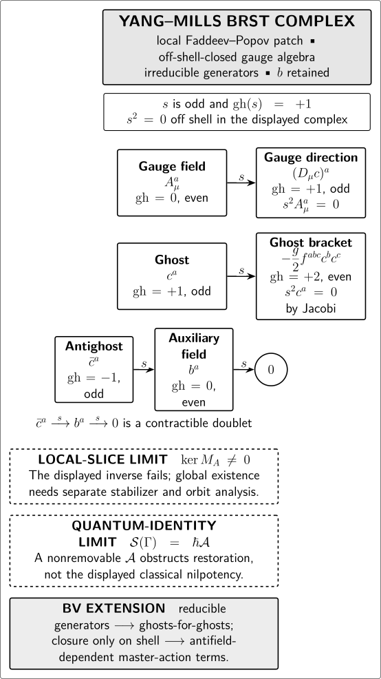
For irreducible Yang–Mills theory with an off-shell-closed algebra, the solid arrows preview a classically nilpotent BRST complex, while the dashed $\ker M_A\neq0$ band marks the separate local-slice failure established on this page. The diagram does not claim that BRST removes Gribov copies, that the slice is global, or that the quantum measure is anomaly free. It is schematic and not to scale.

Open the full-size SVG.

Text equivalent. The diagram assumes a local Faddeev–Popov patch, an irreducible Yang–Mills gauge algebra that closes off shell, and retention of the auxiliary field $b$. Its differential $s$ is odd, has $\operatorname{gh}(s)=+1$, and obeys $s^2=0$ off shell in the displayed complex. The solid arrows map the even gauge field $A_\mu^a$ of ghost number zero to the odd gauge direction $(D_\mu c)^a$ of ghost number one. They map the odd ghost $c^a$ to $sc^a=-\frac{g}{2}f^{abc}c^bc^c$, an even expression of ghost number two; $s^2c^a=0$ follows from the Jacobi identity. They also form the contractible doublet $\bar c^a\mapsto b^a\mapsto0$, from the odd antighost of ghost number $-1$ to the even auxiliary field of ghost number zero.

A separate dashed band states that $\ker M_A=\ker\mathcal M_A\neq0$ invalidates the local Faddeev–Popov inverse and requires stabilizer and orbit analysis. The quantum-identity band displays $\mathcal S(\Gamma)=\hbar\mathcal A$: a nonremovable $\mathcal A$ obstructs restoration of the quantum identity without negating the displayed classical nilpotency. The final BV band says that reducible generators require ghosts-for-ghosts, while an algebra closing only on shell requires antifield-dependent master-action terms. Only the local-slice band is developed here; the following pages own the arrows and their extensions.

Restricting a nonperturbative integral to $\Omega_1^\circ$ introduces a configuration-space boundary. The familiar integration-by-parts argument for a Ward identity then requires proof that the relevant flow preserves the domain, or an explicit treatment of the boundary term. A naive restriction does not supply that proof.

Current nonperturbative status, evidence checked through 8 August 2026. Restriction to the first region is not a settled construction of the global quotient. A peer-reviewed 2026 research paper treats Gribov–Zwanziger restriction and Serreau–Tissier weighted averaging over copies as distinct active continuum strategies and studies a relation between them; it does not establish either as the unique global solution Carmo Terin 2026, §§ 1–2.2, final PDF, printed pp. 1–3. Their dynamical, functional, and lattice consequences belong to the downstream pages listed below.

Common pitfalls

Calling every zero mode a copy. A stabilizer zero mode generates no field displacement. A non-stabilizer zero mode generates a tangent direction, but a finite second intersection still requires solving the nonlinear orbit equation.

Assuming copies force zero modes at their endpoints. The offset-circle example has two transverse copies with nonzero, opposite Jacobians. A zero may occur elsewhere in a controlled family, but that is a separate spectral-flow statement.

Equating the first region with a fundamental domain. Positivity makes the orbit-norm Hessian locally positive. The first region can still contain several representatives from one orbit; the fundamental modular region and a global quotient are stronger constructions.

Inferring operator positivity from the determinant sign. A determinant is a product of eigenvalues at a regulator. An even number of negative eigenvalues can give a positive product, while $\mathcal M_A>0$ requires every relevant eigenvalue to be positive.

Dividing out a charged boundary transformation. Copy classification uses the declared redundancy group. A boundary-nontrivial transformation that carries charge is not redundant merely because it preserves a boundary condition.

Generalizing the Maxwell result to every Abelian gauge problem. The uniqueness proof used a trivial bundle, the based identity component, a connected bounded region, a linear Coulomb condition, and Dirichlet data. Changing any of those ingredients can restore residual transformations or topological sectors.

Treating the Gribov horizon as a causal horizon. It is a spectral boundary in configuration space where an elliptic operator develops a zero eigenvalue. It is not a spacetime light cone, event horizon, or causal surface.

Claiming that BRST cures copies or that copies prove confinement. Local BRST nilpotency and global slice uniqueness are different tests. Gribov copies motivate nonperturbative programs, but their existence alone proves no confinement mechanism.

Check your understanding

1. Classify the offset-circle intersections. For each of $r>a$, $r=a$, and $r<a$, count the roots and compute $M$. A sound response distinguishes two transverse copies, one non-stabilizer tangency, and a missed orbit.

2. Test the Maxwell uniqueness proof. Repeat the energy argument with Neumann rather than Dirichlet data. A sound response identifies the constant kernel and explains why the redundancy group or residual quotient must be specified before claiming uniqueness.

3. Read a Yang–Mills zero mode. Suppose $\mathcal M_A\epsilon=0$ on the based Dirichlet domain. A sound response concludes loss of the local inverse and a tangent orbit direction, but does not claim a finite second representative without solving $F[A^g]=0$.

4. Separate BRST from the slice. Explain why the Jacobi-identity proof of $s^2=0$ and the invertibility test for $M_A$ are independent. A sound response also names the extra domain, regulator, measure, and anomaly conditions needed for a quantum Ward identity.

Continue beyond the local patch

For algebraic control inside a valid patch, continue to The BRST Differential and Gauge-Fixed Complex. That construction is local; it is not a global cure for copies.

For nonperturbative functional consequences, continue to Gauge Fixing, BRST, and Gribov Issues. For lattice implementation and copy-dependent correlators, continue to Gauge Fixing, Gribov Copies, and Gauge-Dependent Correlators.

For theorem-level geometry, use Local Slices, Gauge Fixing, and Faddeev–Popov Geometry and The Gribov–Singer Global Gauge-Fixing Obstruction. For singular orbit spaces and stabilizers, use Orbit Spaces, Stabilizers, and Stratified Quotients.

References

• Assanioussi, Mehdi, Jerzy Kowalski-Glikman, Ilkka Mäkinen, and Ludovic Varrin. “On the Covariant Formulation of Gauge Theories with Boundaries.” Classical and Quantum Gravity 41, no. 11 (2024): 115007. DOI. Open PDF, arXiv v2.
• Carmo Terin, Rodrigo. “Towards a Unified Viewpoint of Gribov–Zwanziger and Serreau–Tissier Gauge Fixing.” Physics Letters B 875 (2026): 140302. DOI. Final open record. Open PDF.
• Fuster, Andrea, Marc Henneaux, and Axel Maas. “BRST-Antifield Quantization: A Short Review.” International Journal of Geometric Methods in Modern Physics 2, no. 5 (2005): 939–964. DOI. Open PDF, arXiv v2.
• Gribov, V. N. “Quantization of Non-Abelian Gauge Theories.” Nuclear Physics B 139, nos. 1–2 (1978): 1–19. DOI.
• Singer, I. M. “Some Remarks on the Gribov Ambiguity.” Communications in Mathematical Physics 60, no. 1 (1978): 7–12. DOI. Open PDF.
• Srednicki, Mark. Quantum Field Theory. Cambridge: Cambridge University Press, 2007. DOI. Author page and errata.
• Vandersickel, Nele, and Daniel Zwanziger. “The Gribov Problem and QCD Dynamics.” Physics Reports 520, no. 4 (2012): 175–251. DOI. Open PDF, arXiv v2.
• Vassilevich, D. V. “Heat Kernel Expansion: User’s Manual.” Physics Reports 388, nos. 5–6 (2003): 279–360. DOI. Open PDF, arXiv v3.
• Zinn-Justin, Jean. Quantum Field Theory and Critical Phenomena. 5th ed. Oxford: Oxford University Press, 2021. DOI.