Proper and Improper Gauge Transformations

An allowed gauge transformation is proper only when, on the declared boundary phase space, its complete differentiable generator has zero differential along every admitted variation and the identity-connected direction is declared redundant. If that differential is nonzero, the transformation acts physically and is improper, or charged. Neither the boundary value of the gauge parameter, its survival after gauge fixing, nor the value of a charge on one state decides the question.

This page develops that first classification for Maxwell and compact Yang–Mills theory on a region with a smooth finite boundary, using fixed, field-independent gauge parameters.

Required background. Gauge Orbits, Gauss Constraints, and Stabilizers supplies the Gauss-orbit and complete-generator conventions; Boundaries, Flux, and Boundary Ward Identities separates timelike Ward flux from charge on a spatial cut; and Presymplectic Systems and the Covariant Phase-Space Ambiguity Map supplies the contraction and null-direction test. Global integrability, reference choices, field-dependent parameters, flux prescriptions, and charge algebras begin on the following pages.

Declare the boundary problem first

Let $\Sigma$ be an oriented spatial hypersurface with $S=\partial\Sigma$, let $\mathcal P$ be its canonical field space, and let $\mathcal P_{\mathrm G}\subset\mathcal P$ be the Gauss-constraint surface. Before labeling a gauge parameter $\epsilon$, one must fix four pieces of data:

1. the action, including the boundary and corner terms needed for its variational principle;
2. the field and bundle sector, the boundary conditions, and hence the admitted tangent variations $\delta\Phi$;
3. the class of parameters whose transformations preserve all those data; and
4. the orientation and any boundary contribution to the presymplectic form.

Call the resulting group of allowed transformations $\mathcal G_{\mathrm{adm}}$. Admissibility comes before charge: a transformation that fails to preserve the chosen field space or boundary condition is not a symmetry of that boundary problem. Conversely, preserving the boundary condition establishes only admissibility; it does not establish that the transformation is redundant. Boundary conditions enter the definition of the phase space in precisely this way Harlow and Wu 2020, §§ 2.1–2.4, pp. 7–23, Open PDF.

The subgroup eventually divided out is smaller. Denote by $\mathcal G_0\subseteq\mathcal G_{\mathrm{adm}}$ the identity-connected transformations whose completed generator has zero differential everywhere on the allowed part of $\mathcal P_{\mathrm G}$ and which the theory declares to be redundancies. When this subgroup is normal and the action descends regularly, reduction takes the form $\mathcal P_{\mathrm G}/\mathcal G_0$. Charged boundary transformations stay outside $\mathcal G_0$ and act on the reduced phase space.

The Gauss generator needs a surface completion

Continue the site’s canonical Yang–Mills conventions,

$$\begin{aligned} \Omega_\Sigma &= \int_\Sigma d^3x\, \boldsymbol\delta A_i^a\wedge \boldsymbol\delta E^{ia}, \\ E^{ia} &=F^{i0a}, \\ (D_i\epsilon)^a &= \partial_i\epsilon^a +g f^{abc}A_i^b\epsilon^c, \qquad \mathcal C^a=(D_iE^i)^a, \end{aligned}$$

with $E^{\perp a}=n_iE^{ia}$ for the outward normal to $S$. Smearing the Gauss constraint alone gives

$$G_{\mathrm{bulk}}[\epsilon] = -\int_\Sigma d^3x\, \epsilon^a\mathcal C^a.$$

For fixed $\epsilon$, its variation contains the boundary remainder

$$\begin{aligned} \boldsymbol\delta G_{\mathrm{bulk}}[\epsilon] &= \int_\Sigma d^3x\, (D_i\epsilon)^a\boldsymbol\delta E^{ia} - g\int_\Sigma d^3x\, f^{abc}E^{ib}\epsilon^c\boldsymbol\delta A_i^a \\ &\quad -\int_S d^2S\, \epsilon^a\boldsymbol\delta E^{\perp a}. \end{aligned}$$

If the phase space allows $E^\perp$ to vary, the last term is uncontrolled. Adding

$$Q_S[\epsilon] = \int_S d^2S\, \epsilon^aE^{\perp a}$$

cancels it and produces the complete functional

$$\begin{aligned} G[\epsilon] &= G_{\mathrm{bulk}}[\epsilon]+Q_S[\epsilon] \\ &= \int_\Sigma d^3x\, E^{ia}(D_i\epsilon)^a \\ &= -\int_\Sigma d^3x\, \epsilon^a(D_iE^i)^a + \int_S d^2S\, \epsilon^aE^{\perp a}. \end{aligned}$$

A functional is differentiable here when its first variation is finite and has no unprescribed boundary remainder for every admitted tangent variation. This is a statement about the chosen phase space: if the boundary condition instead fixes $E^\perp$, then $\boldsymbol\delta E^\perp=0$ and the bulk functional is already differentiable, while $Q_S$ is constant on each connected component of phase space. The canonical constraint and its action are reviewed in Tong 2018, § 2.2.1, pp. 40–42, official full-notes PDF.

On $\mathcal P_{\mathrm G}$ the bulk constraint vanishes, so the completed generator reduces to its surface term,

$$G[\epsilon]\big|_{\mathcal P_{\mathrm G}} =Q_S[\epsilon].$$

This equality does not mean that a boundary value is automatically a charge. It says that, once the transformation is admitted and the generator is complete, the boundary functional carries the remaining test.

Proper, improper, and unresolved directions

With the site convention $\iota_{R_\epsilon}\Omega_\Sigma=\boldsymbol\delta G[\epsilon]$, define on the Gauss surface

$$\eta_\epsilon(\delta) := \bigl(\iota_{R_\epsilon}\Omega_\Sigma\bigr)(\delta) = \boldsymbol\delta G[\epsilon](\delta), \qquad \delta\in T\mathcal P_{\mathrm G}.$$

The displayed $\Omega_\Sigma$ and $G[\epsilon]$ fix the canonical representative used in this test. In a general covariant construction, the symplectic-potential, improvement, and corner representatives must likewise be fixed—or their dependence carried—before the pairing is classified. Changing that prescription requires repeating the test; the next page tracks this dependence explicitly. For the fixed representative here, the first fork is exact.

• If $\eta_\epsilon(\delta)=0$ for every admitted $\delta$, the generator is constant on each connected component. Its state-independent constant may be normalized to zero. An identity-connected direction is a proper or null candidate, and becomes a redundancy when the theory includes it in $\mathcal G_0$.
• If an explicit differentiable $G[\epsilon]$ exists and $\eta_\epsilon(\delta)\neq0$ for at least one admitted $\delta$, then $R_\epsilon$ is not a null direction. It acts as an improper or charged boundary transformation and must not be quotiented away.
• If no finite, well-defined completion exists, there is no Hamiltonian generator on this phase space. If only a candidate surface one-form is known, its global exactness is still unresolved; calling it $\boldsymbol\delta H_\epsilon$ does not prove that a global $H_\epsilon$ exists.

This terminology is used in a particularly sharp surface-one-form form in Barnich and Compère 2008, § 4.2, pp. 14–15, Open PDF. Their setting is asymptotic; the finite-boundary criterion above is the corresponding presymplectic test on a declared phase space. Gauge invariance of $\Omega_\Sigma$ is weaker than degeneracy along $R_\epsilon$: invariance says the form is preserved, whereas properness requires its contraction with the direction to vanish Assanioussi et al. 2024, §§ 3.1–3.4, pp. 13–18, Open PDF.

Several nearby labels answer different questions:

Label	Question it answers	What it does not imply
Admissible	Does the transformation preserve the declared boundary problem?	That it is null or Hamiltonian
Residual	Does it also preserve a chosen gauge-fixing condition?	That it is proper, improper, or physical
Proper	Does the completed generator have zero differential for every admitted variation, with the identity-connected direction declared redundant?	That the parameter must vanish at $S$
Improper	Does an admitted transformation act through a nontrivial differentiable generator?	That it is disconnected from the identity
Large	Is the transformation disconnected or topologically nontrivial relative to the chosen group?	That it has nonzero boundary charge
Stabilizer	Does $R_\epsilon$ vanish at a particular configuration?	That the same direction is null throughout phase space

Thus “small/large” and “proper/improper” are independent distinctions. An identity-connected transformation can be improper, while a disconnected one can have vanishing charge in a particular theory. In Yang–Mills theory a reducibility parameter obeying $D\chi=0$ is a stabilizer-like zero mode; that is distinct from a nonzero orbit direction whose presymplectic pairing vanishes Riello 2021, § 4.4, p. 24, Open PDF.

The chapter-wide decision map

The diagram below records the whole chapter sequence. This page covers the declaration, admissibility, generator completion, and null/non-null split. Representative dependence, global exactness, flux, algebra, and optional edge extensions are shown only as forward tests and are developed on the following pages.

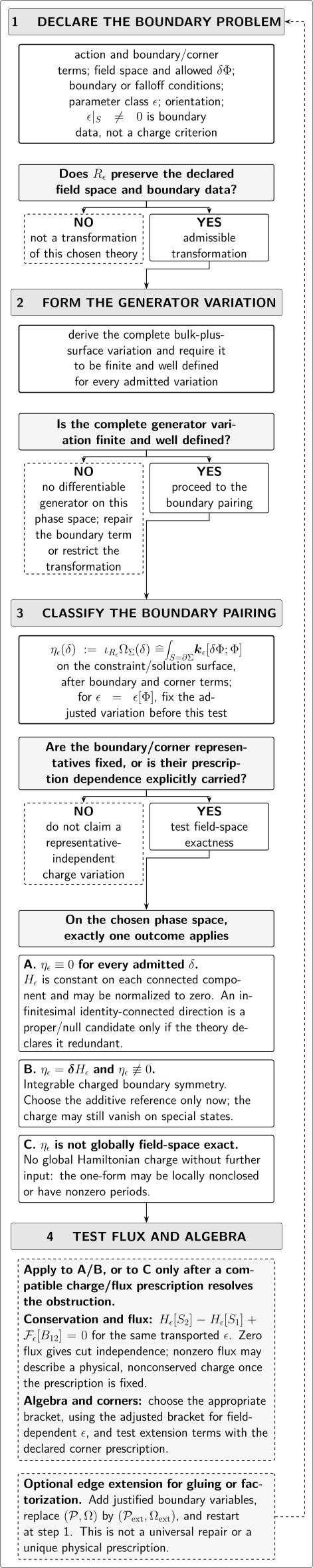
A parameter acquires physical meaning through the declared phase space and its generator, not through $\epsilon|_S$ alone. This page stops after forming $\eta_\epsilon=\iota_{R_\epsilon}\Omega_\Sigma$ and deciding whether it vanishes. The lower stages preview the later tests: a nonzero one-form must be globally exact before it defines $H_\epsilon$; conservation and algebra are separate questions; and an edge extension changes the phase space, so the classification restarts. In the displayed flux convention, positive $\mathcal F_\epsilon[B_{12}]$ lowers $H_\epsilon$ from $S_1$ to $S_2$. The diagram is schematic and not to scale.

The complete text equivalent is:

Stage	Required test	Valid conclusion	Scope
Declare	Fix the action and boundary/corner terms, fields, admitted variations, boundary conditions, parameter class, and orientation	The boundary problem is defined	This page
Admit	Check that $R_\epsilon$ preserves every declared datum	Admissible, or else not a transformation of this theory	This page
Form the generator	Derive the complete bulk-plus-surface variation and require it to be finite and well defined for every admitted variation	A candidate generator one-form exists, or the construction stops	This page
Fix representatives	Fix the symplectic-potential, improvement, and corner representatives, or carry their dependence	The candidate has a declared prescription	Canonical choice above; general ambiguity next page
Null outcome	Test $\eta_\epsilon(\delta)=0$ for every admitted $\delta$	The generator is componentwise constant; an identity-connected direction may be declared proper	First fork here
Charged outcome	Test whether $\eta_\epsilon=\boldsymbol\delta H_\epsilon$ globally and $\eta_\epsilon\not\equiv0$	An integrable charged boundary symmetry	Exactness next page
Nonexact outcome	Test local closure and periods on field space	No global Hamiltonian charge without further input	Next page
Field-dependent parameter	Define the adjusted variation before any of the three outcomes	Field dependence changes the prescription, not the list of outcomes	Next page
Flux and algebra	For an existing or repaired charge, test $H_\epsilon[S_2]-H_\epsilon[S_1]+\mathcal F_\epsilon[B_{12}]=0$ and then the appropriate bracket	Conservation and algebra are independent of integrability	Later pages
Optional extension	Justify new boundary variables, replace $(\mathcal P,\Omega)$ by $(\mathcal P_{\mathrm{ext}},\Omega_{\mathrm{ext}})$, and restart	An extension may solve a specified gluing problem; it is not universal	Edge-mode page

Maxwell theory with several boundary components

Now take $M=\mathbb R\times\Sigma$ in source-free Maxwell theory, with $\Sigma$ compact and connected, and write its entire boundary as $S=\partial\Sigma=\bigsqcup_{a=1}^N S_a$. Fix the pullback of $A$ to the timelike wall $\Gamma=\mathbb R\times S$. An admitted gauge transformation $A\mapsto A+d\lambda$ must obey

$$\iota_\Gamma^*(d\lambda)=0, \qquad \lambda|_{S_a}=c_a,$$

so the boundary value is constant on each connected component. The completed canonical generator is

$$\begin{aligned} G[\lambda] &= \int_\Sigma d^3x\,E^i\partial_i\lambda \\ &= -\int_\Sigma d^3x\, \lambda\,\partial_iE^i + \sum_{a=1}^N c_a\Phi_a, \\ \Phi_a &:= \int_{S_a}d^2S\,E^\perp. \end{aligned}$$

On the Gauss surface,

$$Q[\lambda] = \sum_a c_a\Phi_a, \qquad \eta_\lambda(\delta) = \sum_a c_a\boldsymbol\delta\Phi_a.$$

This is the finite-boundary Maxwell charge derived covariantly in Harlow and Wu 2020, § 3.3, pp. 26–27, Open PDF. The electric flux $\Phi_a$ through a spatial cut is the canonical charge here; it is not the timelike matter- or boundary-current flux that appears in the preceding Ward balance law.

Source-free Gauss law and outward orientation give

$$\sum_a\Phi_a=0, \qquad \sum_a\boldsymbol\delta\Phi_a=0.$$

The consequences expose why $\lambda|_S$ is not a classification rule.

• Diagonal constant. If every $c_a=c$, then $Q[\lambda]=c\sum_a\Phi_a=0$. The common mode is null in this source-free phase space even though its boundary value need not vanish.
• Relative constants. If the $c_a$ differ, then only their differences survive. For two components, $Q[\lambda]=(c_1-c_2)\Phi_1$. This direction is improper whenever admitted variations can change the relative flux, because then $\eta_\lambda\neq0$.
• Fixed-flux phase space. In a different well-posed boundary problem that imposes $\boldsymbol\delta\Phi_a=0$ for every component, $\eta_\lambda=0$ even for nonzero, unequal $c_a$. The same boundary parameter is now a null candidate because the phase space has changed.

With charged matter, the diagonal conclusion must be recomputed: Gauss law relates total electric flux to bulk charge, and a constant $U(1)$ parameter also acts on the matter fields. It is then neither the pure-Maxwell stabilizer nor automatically proper.

Orbit, charge, and gauge-fixed descriptions agree

The same Maxwell classification looks different in three descriptions, but the test is unchanged.

Description	Object to compute	Correct conclusion
Orbit	The identity-connected null subgroup $\mathcal G_0$	Quotient the based and other declared null directions; retain relative boundary transformations when their flux pairing is nonzero
Generator	$\eta_\lambda=\boldsymbol\delta Q[\lambda]=\sum_a c_a\boldsymbol\delta\Phi_a$	Zero for every admitted variation means proper candidate; nonzero somewhere means a charged action
Coulomb gauge	Residual parameters satisfying $\Delta\lambda=0$ with the admitted boundary data	The harmonic residual still has to pass the original boundary and generator tests

On a connected bounded domain, equal boundary constants have the constant harmonic extension and $d\lambda=0$; in pure Maxwell this is a stabilizer. Unequal constants on different components have a nonconstant harmonic extension and survive Coulomb gauge, but “residual” says only that the gauge slice is preserved. Whether such a residual transformation is proper or charged is still decided by $\sum_a c_a\boldsymbol\delta\Phi_a$.

Common failure modes

Using the bulk constraint as the complete generator. Integration by parts exposes a surface variation. Add the boundary completion or state boundary conditions that make the remainder vanish before classifying the direction.

Classifying by the boundary value of the parameter. A nonzero value may be inadmissible, null because the conjugate flux is fixed, or charged because that flux varies. Vanishing at $S$ is sufficient in the elementary canonical Maxwell example, but it is not the definition in a theory with additional boundary symplectic data.

Equating residual with physical. A residual transformation preserves a gauge condition. Properness instead asks whether the completed generator has zero differential on the original admitted phase space.

Testing the value on one state. The equation $G[\epsilon]=0$ at one point does not imply $\boldsymbol\delta G[\epsilon]=0$ for every admitted variation. Conversely, a constant nonzero value can be removed by a reference normalization.

Equating invariance with degeneracy. The condition $\mathcal L_{R_\epsilon}\Omega_\Sigma=0$ says that the transformation preserves the presymplectic form. Properness requires the stronger contraction condition $\iota_{R_\epsilon}\Omega_\Sigma=0$ on the constraint surface.

Equating a stabilizer with a proper direction. A stabilizer satisfies $R_\epsilon(z)=0$ at one configuration $z$. A proper direction is null under the presymplectic pairing throughout the declared region of phase space and is included in the redundant subgroup.

Check your understanding

1. Vary the bulk Maxwell constraint $G_{\mathrm{bulk}}[\lambda]=-\int_\Sigma\lambda\,\partial_iE^i$ and identify the term that prevents differentiability when $E^\perp$ varies.
2. Let $S=S_1\sqcup S_2$ and impose source-free Gauss law. For $c\neq0$, classify boundary data $(c_1,c_2)=(c,c)$ and $(c,-c)$ when $\Phi_1$ may vary.
3. In Coulomb gauge, explain why $\Delta\lambda=0$ does not decide whether a residual transformation is proper.

Solutions

For fixed $\lambda$, integration by parts gives

$$\boldsymbol\delta G_{\mathrm{bulk}}[\lambda] = \int_\Sigma d^3x\, (\partial_i\lambda)\boldsymbol\delta E^i - \int_S d^2S\, \lambda\boldsymbol\delta E^\perp.$$

The last term is canceled by $\boldsymbol\delta Q[\lambda] =\int_S\lambda\boldsymbol\delta E^\perp$ unless the allowed variations already set it to zero.

For two components, $\Phi_2=-\Phi_1$, so

$$Q[\lambda] =(c_1-c_2)\Phi_1.$$

The diagonal data $(c,c)$ are null. For $c\neq0$, the relative data $(c,-c)$ give $Q=2c\Phi_1$ and are charged when $\boldsymbol\delta\Phi_1$ is admitted.

Finally, $\Delta\lambda=0$ only says that $A_i+\partial_i\lambda$ remains in Coulomb gauge. One must separately impose the original boundary condition and evaluate $\eta_\lambda=\sum_a c_a\boldsymbol\delta\Phi_a$; the result can be null or charged depending on the admitted flux variations.

Where the classification continues

Surface Charges, Integrability, and Ambiguities tests local closure, global periods, improvements, corner representatives, additive normalization, conservation, and the adjusted variation for field-dependent parameters. Charge Algebras, Central Terms, and Corners then tests the bracket and possible extensions. Edge Modes, Subregions, and Factorization asks whether a specified gluing problem justifies extending the phase space, while Asymptotic Symmetry, Soft Limits, and the Boundary Interface supplies the extra falloff and limiting data required at infinity.

References

• Assanioussi, Mehdi, Jerzy Kowalski-Glikman, Ilkka Mäkinen, and Ludovic Varrin. “On the Covariant Formulation of Gauge Theories with Boundaries.” Classical and Quantum Gravity 41 (2024): 115007. DOI. Open PDF
• Barnich, Glenn, and Geoffrey Compère. “Surface Charge Algebra in Gauge Theories and Thermodynamic Integrability.” Journal of Mathematical Physics 49 (2008): 042901. DOI. Open PDF
• Harlow, Daniel, and Jie-qiang Wu. “Covariant Phase Space with Boundaries.” Journal of High Energy Physics 2020, no. 10 (2020): 146. DOI. Open PDF
• Riello, Aldo. “Edge Modes without Edge Modes.” arXiv:2104.10182 (2021). arXiv record. Open PDF
• Tong, David. Gauge Theory. Cambridge Part III Mathematical Tripos lecture notes, 2018. Official course page. Official PDF