Operators, Boundaries, and Relative Topological Theories

Topological line data do not, by themselves, determine what happens at a boundary. Fusion and braiding describe how bulk operators compose and move; a physical boundary additionally declares which operators may end or condense, what boundary-changing junctions exist, and how the remaining operators act. An interface is the same question for two bulk theories after folding one side. A relative theory is different again: its partition function is valued in a state space supplied by a theory in one higher dimension, and becomes a number only after a compatible pairing or trivialization.

This page makes those distinctions explicit in compact bosonic Abelian Chern–Simons theory, compact $BF_N$, and finite Dijkgraaf–Witten theory. The default Abelian Chern–Simons domain is a closed oriented three-dimensional bulk with a chosen quantum framing convention and an even, nonsingular, symmetric integral matrix $K$. Boundaries and interfaces are opened only after their orientation, tangential structure, and boundary data are stated. Odd $K$ requires spin refinements and is not silently included in the bosonic quadratic formulas below.

Required background. Abelian Chern–Simons Theory supplies the discriminant group and its braid, twist, and state-space data. Boundaries, Interfaces, and Domain Walls supplies the geometric folding convention. Fusion, Junctions, and Endpoints separates a fusion rule from the junction space that realizes it. Helpful background. Edge Modes, Subregions, and Factorization explains why gluing matches shared data and reduces only once.

Fusion, braiding, and spin come from K inverse

For the even nonsingular $K$ theory, the bulk Wilson-line classes form

$$\mathcal A=\mathbb Z^r/K\mathbb Z^r.$$

The class of $\ell\in\mathbb Z^r$ will be written $[\ell]$. Fusion is addition,

$$[\ell]\otimes[m]=[\ell+m],$$

and the protected fusion space in this Abelian model is

$$V_{\ell m}^{\ \ n} \cong \begin{cases} \mathbb C, & [n]=[\ell+m],\\ 0, & \text{otherwise}. \end{cases}$$

Multiplicity one does not make the associator trivial: changing representatives of $\mathcal A$ can leave nontrivial coherent phases at successive junctions. The complete associator belongs to the categorical handoff, not to an arithmetic fusion slogan.

The inverse matrix gives the nondegenerate discriminant pairing and, for even $K$, its quadratic refinement:

$$\begin{aligned} b([\ell],[m]) &= \ell^{\mathsf T}K^{-1}m \pmod 1, \\ q([\ell]) &= \frac12\ell^{\mathsf T}K^{-1}\ell \pmod 1. \end{aligned}$$

In the fixed positive-orientation convention,

$$M_{\ell m} = \exp\!\bigl(2\pi i\,b([\ell],[m])\bigr), \qquad \theta_\ell = \exp\!\bigl(2\pi i\,q([\ell])\bigr).$$

Here $M_{\ell m}$ is a full mutual braid, not one exchange, and $\theta_\ell$ uses a positive unit framing twist. Orientation reversal complex-conjugates both phases. Kapustin and Saulina derive the line quotient, fusion channels, braiding, and the possible associator phases in Kapustin and Saulina 2011, §§ 3.1–3.2, arXiv v2, printed pp. 3–8, PDF.

The following schematic packages the four operations controlled by the same discriminant data. It deliberately stops before boundaries: deciding which lines can terminate is new information.

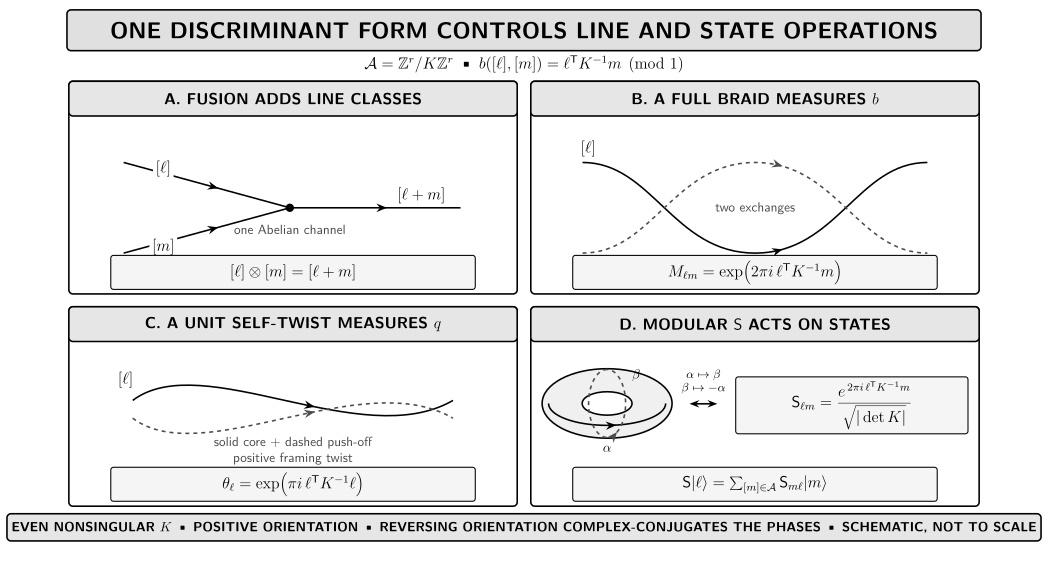
For an even nonsingular $K$, the discriminant group $\mathcal A=\mathbb Z^r/K\mathbb Z^r$ supplies the line labels and fusion, while $K^{-1}$ supplies their nondegenerate bilinear pairing. The positive full braid gives $M_{\ell m}$, a positive unit framing twist gives $\theta_\ell$, and the normalized pairing gives the orientation-preserving torus modular map $(\alpha,\beta)\mapsto(\beta,-\alpha)$. Reversing orientation complex-conjugates the phases. The diagram is schematic, not to scale, and does not extend the bosonic quadratic formula to odd $K$ or assert a non-Abelian coherence or boundary classification.

A gapped boundary selects condensable lines

For a subgroup $L\subset\mathcal A$, define its orthogonal complement

$$L^\perp = \left\{ a\in\mathcal A \ \middle|\ b(a,\ell)=0 \text{ for every }\ell\in L \right\}.$$

In the controlled bosonic Abelian class considered here, the elementary topological-boundary datum is a Lagrangian subgroup satisfying

$$q|_L=0, \qquad L=L^\perp.$$

The first condition says that the condensed lines have trivial topological spin; it also makes their mutual braiding trivial. The second says that the condensate is maximal: every line that braids trivially with it is already in it. Since $b$ is nondegenerate,

$$\lvert L\rvert^2=\lvert\mathcal A\rvert.$$

A bulk line in $L$ can end on this boundary. Unscreened elementary boundary line charges are represented by $\mathcal A/L$, while a junction between two boundary types $L_1$ and $L_2$ carries charge in

$$\mathcal A/(L_1+L_2).$$

These quotient statements record which topological charge remains after the two boundary condensates are available. They do not determine every junction amplitude or associator.

The Lagrangian criterion is a powerful finite test, but it has a domain. Its use for an arbitrary abstract Lagrangian subgroup is a supported construction in this model, not a theorem that classifies every boundary of every TQFT. A purely topological vacuum boundary in the Abelian Chern–Simons construction also requires cancellation of the chiral gravitational obstruction; in particular the controlled $K$-matrix construction has $\operatorname{sign}(K)=0$. Conversely, failure of this finite test does not forbid a gapless edge or a boundary with additional degrees of freedom. For example,

$$K=(2), \qquad \mathcal A=\mathbb Z_2, \qquad q(1)=\frac14 \pmod 1$$

has no Lagrangian subgroup: $\lvert\mathcal A\rvert=2$ is not a square and the nontrivial line is not bosonic. This rules out the gapped topological vacuum boundary in the stated class, not every possible physical boundary. Conversely, the positive-definite $E_8$ Cartan matrix is even and unimodular, so $\mathcal A=0$ and $L=\{0\}$ passes the finite test vacuously, while $\operatorname{sign}(K)=8$ still obstructs a topological boundary to the vacuum. The anyon test cannot see that chiral gravitational response. Kapustin and Saulina give the signature ceiling and Lagrangian-subgroup construction in Kapustin and Saulina 2011, § 4.1, printed pp. 10–11, and §§ 5.1 and 6.2, printed pp. 15–17 and 30–33, arXiv v2 PDF.

Compact BF has two complementary elementary boundaries

Three-dimensional compact $BF_N$ theory is the off-diagonal Chern–Simons theory

$$K_{BF} = \begin{pmatrix} 0&N\\ N&0 \end{pmatrix}, \qquad N\in\mathbb Z_{>0}.$$

Its bulk line group and quadratic data are

$$\begin{aligned} \mathcal A_{BF} &= \mathbb Z_N^{\,e}\times\mathbb Z_N^{\,m}, \\ q(e,m) &= \frac{em}{N} \pmod 1, \\ b\bigl((e,m),(e',m')\bigr) &= \frac{em'+me'}{N} \pmod 1. \end{aligned}$$

The two coordinate subgroups

$$L_e=\{(e,0)\}, \qquad L_m=\{(0,m)\}$$

are Lagrangian. The electric boundary absorbs the $e$-lines and the magnetic boundary absorbs the $m$-lines. The dyon $(1,1)$ at $N=2$ has $q(1,1)=1/2$ and cannot be added to an ordinary bosonic condensate.

The quotient at an elementary Abelian boundary-changing junction gives an immediate finite check:

$$\dim\mathcal H_{\mathrm{cyl}}(L_1,L_2) = \left| \mathcal A_{BF}/(L_1+L_2) \right|.$$

Thus

$$\dim\mathcal H_{\mathrm{cyl}}(L_e,L_e)=N, \qquad \dim\mathcal H_{\mathrm{cyl}}(L_e,L_m)=1.$$

The first cylinder retains one unscreened magnetic label. The second has both electric and magnetic condensates available at its two ends, so no nontrivial bulk label survives. This is a boundary-state count, not the closed-surface value $\dim\mathcal H(T^2)=N^2$. The quotient and interval reduction are developed in Kapustin 2014, §§ II–IV, arXiv v1, printed pp. 1–4, especially the discussion of $\mathcal A/(L_1+L_2)$, PDF.

At the action level, in the Lorentzian phase convention, with

$$S_{BF} = \frac{N}{2\pi}\int_M B\wedge dA,$$

the transformation $B\mapsto B+d\beta$ gives

$$\Delta_\beta S_{BF} = \frac{N}{2\pi}\int_{\partial M}\beta\wedge dA.$$

A physical boundary must therefore restrict boundary gauge transformations, impose a compatible polarization, add a boundary counterterm, or supply boundary degrees of freedom with the inverse variation. The bulk action alone does not select between $L_e$ and $L_m$.

Folding turns an interface into a boundary problem

An interface from $\mathcal T_1$ to $\mathcal T_2$ becomes, after folding, a boundary condition for

$$\mathcal T_1\otimes\overline{\mathcal T_2}.$$

For Abelian Chern–Simons theories this gives

$$K_{\mathrm{fold}} = K_1\oplus(-K_2), \qquad \mathcal A_{\mathrm{fold}} = \mathcal A_1\times\mathcal A_2,$$

with

$$q_{\mathrm{fold}}(a_1,a_2) = q_1(a_1)-q_2(a_2).$$

The minus sign is the orientation reversal of the second theory. It is not optional convention data once the coorientation of the original interface is fixed.

For two copies of the same theory, the diagonal subgroup

$$L_\Delta=\{(a,a)\mid a\in\mathcal A\}$$

is Lagrangian in the folded theory. It is the transparent identity wall: every line crosses with the same label. More generally, if

$$\varphi:\mathcal A_1\longrightarrow\mathcal A_2$$

is an isomorphism preserving $q$, then its graph

$$\Gamma_\varphi=\{(a,\varphi(a))\}$$

is Lagrangian in $\mathcal A_1\times\mathcal A_2$ with the folded quadratic form. This verifies the finite braid-and-spin test for an invertible Abelian wall. A general Lagrangian subgroup of the folded data can describe a condensation wall and need not be invertible; composing such walls may decompose into several channels. Full composition, adjunction, and coherence require the module and bimodule structures handed to Mathematical QFT.

The folded Abelian construction is developed in Kapustin and Saulina 2011, § 7.1, arXiv v2, printed pp. 33–35, PDF. Folding is a translation of the interface problem, not a proof that a proposed wall is local, gapped, topological, or invertible.

A sewing cut is not a physical boundary

Suppose a closed spacetime is cut along a spatial manifold $\Sigma$:

$$M=M_2\cup_\Sigma M_1.$$

The cut exposes the full boundary state of the bulk theory, and gluing contracts it:

$$Z(M) = \left\langle Z(M_2),Z(M_1)\right\rangle_{\mathcal H(\Sigma)}.$$

No condensate has been chosen. In finite gauge theory the formula includes the groupoid measure,

$$Z(M) = \sum_{[Q]\in\pi_0\operatorname{Bun}_G(\Sigma)} \frac{ \left\langle Z(M_2;Q),Z(M_1;Q) \right\rangle }{ \lvert\operatorname{Aut}(Q)\rvert }.$$

Replacing that cut by a physical boundary would instead restrict the admissible bundle or line-endpoint data and could add boundary degrees of freedom. It would not reproduce the identity cylinder in general. Fuchs, Schweigert, and Valentino explicitly separate cut-and-paste boundaries from physical boundary conditions in Fuchs, Schweigert, and Valentino 2014, Introduction, arXiv v3, internal printed p. 3, PDF. Freed and Quinn prove the finite-gauge state-space pairing and sewing law in Freed and Quinn 1993, § 2, printed pp. 443–446, especially eqs. (2.1), (2.11), and (2.17)–(2.18) and Theorem 2.13, current arXiv v3 PDF.

The same distinction is visible in compact $BF_N$ without evaluating a continuum path integral. Let

$$A_g=H^1(\Sigma_g;\mathbb Z_N), \qquad \lvert A_g\rvert=N^{2g},$$

and use the perfect pairing

$$[b,a] = \left\langle b\smile a,[\Sigma_g]\right\rangle \in\mathbb Z_N.$$

Changing from the $A$- to the $B$-polarization on an artificial cut uses the finite Fourier kernel

$$K_{BA}(b,a) = \frac{1}{\sqrt{\lvert A_g\rvert}} \exp\!\left(\frac{2\pi i}{N}[b,a]\right).$$

Orientation reversal gives $K_{AB}(a',b)=\overline{K_{BA}(b,a')}$. Gluing the two half-cylinders sums the shared residual mode exactly once:

$$\begin{aligned} K_{AA}(a',a) &= \sum_{b\in A_g} K_{AB}(a',b)K_{BA}(b,a) \\ &= \frac{1}{\lvert A_g\rvert} \sum_{b\in A_g} \exp\!\left( \frac{2\pi i}{N}[b,a-a'] \right) \\ &= \delta_{a',a}. \end{aligned}$$

Omitting the normalization from both kernels would leave $\lvert A_g\rvert\delta_{a',a}$ and expose the cut. This Fourier basis change is a sewing operation, not the choice of $L_e$ or $L_m$ at a physical edge.

For Chern–Simons theory the exponentiated action on a manifold with boundary is likewise naturally an element of a boundary line rather than a canonical number. Cutting creates dual line factors on the two sides, and gluing uses their evaluation pairing. Freed gives this action-line and trace law in Freed 1995, § 2, printed pp. 18–19, especially eqs. (2.18), (2.27), and Theorem 2.19(d), arXiv v1 PDF.

A relative theory takes values in another theory

Let $\alpha$ be a $(d+1)$-dimensional field theory. A $d$-dimensional theory relative to $\alpha$ is not merely a theory whose action has a boundary term. It is compatible field-theory data whose value on a closed $d$-manifold $X$ lies in a state space assigned by $\alpha$. In the Freed–Teleman vector convention, $F:\mathbf 1\to\tau_{\le d}\alpha$ gives $Z_F(X)\in\alpha(X)$. Because the bulk filling below prepares that vector, this page uses the explicitly dual functional convention $\widetilde F:\tau_{\le d}\alpha\to\mathbf 1$. For $\partial Y=X$,

$$Z_\alpha(Y)=\alpha(Y)(1)\in\alpha(X), \qquad Z_{\widetilde F}(X)\in\alpha(X)^\vee,$$

so that

$$Z_{\widetilde F}(X)\bigl(Z_\alpha(Y)\bigr) \in\mathbb C.$$

Reversing the boundary orientation interchanges $\alpha(X)$ and its dual. The invariant statement is that the bulk and relative boundary values live in dual targets and pair once.

If $\alpha$ is invertible, $\alpha(X)$ is a line $\mathcal L_\alpha(X)$; this is the anomaly-line situation familiar from inflow. If $\alpha$ is noninvertible, its state space can have dimension greater than one, and the relative partition function is a genuine vector or functional rather than a phase ambiguity. If $\alpha$ is the trivial theory, the target is canonically $\mathbb C$ and $F$ is absolute.

A pointwise linear functional on each $\alpha(X)$ is not enough. The relative assignment must respect bordisms, disjoint unions, orientation, and gluing. Freed and Teleman formulate this as a natural transformation between field theories in Freed and Teleman 2014, Definition 2.1 and § 3, current arXiv v3, printed pp. 3–4 and 8, eqs. (2.2)–(2.4), PDF.

The next figure prevents a common false chain of implications. Extended, relative, and symmetry-TFT data answer different questions; only the solid restriction arrows are automatic.

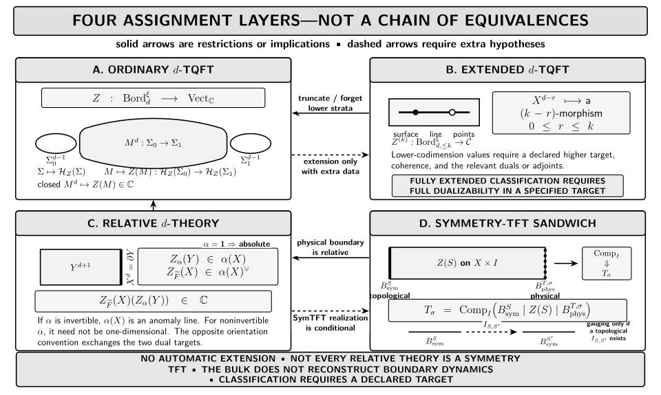
Ordinary, extended, relative, and symmetry-TFT data are related by restrictions and conditional constructions, not by four equivalences. Extension adds lower-codimension assignments in a declared higher target. A relative $d$-theory supplies compatible boundary data relative to an extended $(d+1)$-theory; for an invertible bulk its boundary value pairs with a bulk state in a one-dimensional anomaly line. In the bounded symmetry-TFT sandwich, a suitable topological symmetry boundary and a physical boundary compactified across an interval recover the $d$-dimensional theory. Gauging or condensation changes the symmetry boundary only when the required topological interface exists. The diagram is schematic and does not assert universal symmetry-TFT existence, reconstruct boundary dynamics, or prove a dualizability or classification theorem.

An ordinary unextended TQFT can therefore be the truncation of an extended one, but its state spaces and bordism maps do not prove that such an extension exists. Similarly, every suitable symmetry-TFT physical boundary is relative to its bulk, but a general relative theory need not admit a symmetry-TFT realization. The theorem-level target categories, dualizability hypotheses, and coherence maps are separate mathematical data. The ordinary assignment is the one axiomatized in Atiyah 1988, § 2, printed pp. 177–181, especially axioms (A)–(B) and (1)–(4c), PDF. The bounded sandwich and its conditional change of symmetry boundary are reviewed in Bhardwaj and Schäfer-Nameki 2025, §§ 2.4, 2.6, and 2.7, arXiv v3, printed pp. 21–32, especially Statement 2.1 and eqs. (2.40) and (2.68)–(2.72), PDF. Their construction is a controlled framework, not a universal existence theorem for every relative theory.

First application: one boundary test across three models

The three rows below share a diagnostic, not an equivalence. Each starts with a dynamical topological theory, asks which bulk operators survive or can end, and then distinguishes a physical boundary from an artificial sewing surface.

One boundary-and-interface diagnostic across the three-model topological thread

Model	Bulk operator datum	Gapped boundary datum	Folded interface datum	Gluing or relative signal
Bosonic Abelian Chern–Simons	Discriminant group A with nondegenerate braid pairing b and quadratic refinement q	Lagrangian subgroup L, with q trivial on L and L equal to its orthogonal complement	Lagrangian subgroup of A₁ × A₂ for the difference quadratic form q₁ − q₂	A cut retains the full state space; a physical edge additionally needs anomaly-compatible boundary data
Compact BF at level N	Electric–magnetic group Z_N × Z_N with mutual finite Heisenberg pairing	Electric or magnetic Lagrangian subgroup; same-boundary cylinder has N states, complementary boundaries one	Diagonal gives the transparent wall; more general condensation walls need junction data	Fourier gluing sums one shared residual mode and returns the identity kernel
Finite Dijkgraaf–Witten theory	Flux conjugacy class plus a projective centralizer representation transgressed from the cocycle	Subgroup map together with a cochain trivializing the restricted cocycle, in the elementary class	Subgroup mapping to G₁ × G₂ with a cochain trivializing the folded cocycle difference	Sewing sums boundary bundles with inverse automorphism weight; a physical boundary restricts rather than sums all bundles

For a finite Dijkgraaf–Witten theory $(G,\omega)$, an elementary physical boundary is described by a homomorphism

$$\iota:H\longrightarrow G$$

and a cochain $\vartheta$ satisfying

$$\delta\vartheta=\iota^*\omega.$$

If $[\iota^*\omega]\ne0$, that elementary $H$-boundary does not exist. This is a physical restriction on which finite bundles reach the edge; it is not the cut surface used in the Freed–Quinn sewing sum.

An interface between $(G_1,\omega_1)$ and $(G_2,\omega_2)$ has the folded version of the same test. For

$$\iota=(\iota_1,\iota_2): H\longrightarrow G_1\times G_2,$$

the cochain must obey

$$\delta\vartheta = \iota_1^*\omega_1\, \bigl(\iota_2^*\omega_2\bigr)^{-1}.$$

The inverse is the orientation reversal of the second theory. This formula uses the folded ordering $\mathcal T_1\otimes\overline{\mathcal T_2}$; reversing the interval ordering writes the reciprocal cocycle equation. These subgroup-and-cochain data and their folded interpretation are developed in Fuchs, Schweigert, and Valentino 2014, § 2.5, internal printed pp. 12–13; § 3.2, pp. 17–18, especially eqs. (3.13)–(3.14); and § 3.6, pp. 30–33, arXiv v3 PDF. Their adjacent- interval ordering is the reverse of the folded ordering declared here.

An equal-cardinality check makes the boundary distinction unusually sharp. All three of the following bosonic models have four bulk line classes and

$$\dim\mathcal H(\Sigma_g)=4^g,$$

yet they do not have the same elementary gapped boundaries. For $U(1)_4$,

$$\mathcal A=\mathbb Z_4, \qquad q(a)=\frac{a^2}{8}\pmod 1.$$

The only order-two candidate is $L=\{0,2\}$, but $q(2)=1/2$, so it is not a bosonic Lagrangian subgroup; independently, $\operatorname{sign}(K)=1$ signals the chiral boundary obstruction. For $BF_2$, both $L_e$ and $L_m$ pass. Finally consider the cyclic twist

$$K_{N,r} = \begin{pmatrix} 2r&N\\ N&0 \end{pmatrix}, \qquad q(e,m) = \frac{em}{N}-\frac{r\,m^2}{N^2} \pmod 1,$$

the electric subgroup $L_e$ is always Lagrangian. For $N=2$, $r=0$ is untwisted $BF_2$ and both $L_e$ and $L_m$ are available. For $N=2$, $r=1$,

$$q(0,1)=-\frac14\pmod 1,$$

so the magnetic subgroup fails the bosonic condensation test, even though all three theories have the same line and genus-$g$ state cardinalities. In the elementary bosonic Lagrangian-subgroup class, the counts are therefore zero, two, and one for $U(1)_4$, $BF_2$, and the double-semion twist, respectively. Fusion cardinality does not determine condensability.

Anomaly cancellation is pairing, not erasure

When the one-higher-dimensional theory $\alpha$ is invertible, a background transformation may act on the bulk and boundary factors by inverse phases:

$$\begin{aligned} Z_\alpha[B^g] &= e^{-i\mathcal A(B,g)}Z_\alpha[B], \\ Z_{\widetilde F}[B^g] &= e^{+i\mathcal A(B,g)}Z_{\widetilde F}[B]. \end{aligned}$$

Their pairing is invariant. This does not erase the boundary anomaly; it states that the bulk supplies the inverse anomaly line. A local counterterm can change representatives only when it is globally defined, properly quantized, compatible with all admitted structures, and itself compatible with the boundary. A nontrivial anomaly class is not made zero by calling the boundary relative.

For a noninvertible bulk, anomaly-line language is too narrow: the target state space can have several components, and choosing a boundary condition or symmetry boundary is additional data. That is precisely why the next symmetry-TFT page must be more than an inflow slogan.

What the finite tests do not classify

The calculations above are exact in their stated domains, but several stronger conclusions do not follow.

• A fusion rule and one-dimensional fusion spaces do not determine the associator, junction normalization, or all higher coherence data.
• An isotropic subgroup need not be maximal; only the Lagrangian condition passes the finite gapped-boundary test used here.
• A Lagrangian subgroup does not by itself cancel a chiral gravitational anomaly or prove microscopic boundary realizability.
• Folding does not turn every interface into an invertible wall, and it does not remove orientation, spin, framing, or anomaly data.
• A sewing cut is not a physical boundary. The former retains and sums the complete shared state; the latter selects allowed endpoints or boundary fields.
• A line-valued amplitude on a manifold with boundary is not, by that fact alone, a full relative field theory. Bordism and gluing compatibility are required.
• The finite Abelian Lagrangian-subgroup test does not classify non-Abelian gapped boundaries. Module categories, bimodule defects, full dualizability, and higher coherence belong to the theorem-level handoff.

Check your understanding

1. Verify both BF boundaries

Show directly that $L_e$ and $L_m$ are Lagrangian in $\mathcal A_{BF}=\mathbb Z_N^2$.

Solution

For $(e,0)\in L_e$,

$$q(e,0)=0,$$

so $L_e$ is isotropic. If $(x,y)$ braids trivially with every $(e,0)$, then

$$b\bigl((x,y),(e,0)\bigr)=\frac{ye}{N}=0\pmod 1$$

for every $e$, which forces $y=0$ in $\mathbb Z_N$. Hence $L_e^\perp=L_e$. Exchanging $e$ and $m$ proves $L_m^\perp=L_m$.

2. Test the graph wall

Let $\varphi:\mathcal A_1\to\mathcal A_2$ be an isomorphism that preserves the quadratic refinement. Show that $\Gamma_\varphi$ is Lagrangian in the folded line group.

Solution

For any $a$,

$$q_{\mathrm{fold}}(a,\varphi(a)) = q_1(a)-q_2(\varphi(a)) =0.$$

Thus the graph is isotropic. Since $\varphi$ is an isomorphism,

$$\lvert\Gamma_\varphi\rvert = \lvert\mathcal A_1\rvert = \sqrt{\lvert\mathcal A_1\times\mathcal A_2\rvert}.$$

Nondegeneracy of the folded pairing then gives $\Gamma_\varphi=\Gamma_\varphi^\perp$. This proves the finite Lagrangian test; the existence and coherence of the full wall theory are additional requirements.

3. Find the failed identity

In the $BF_N$ Fourier gluing calculation, omit the factor $\lvert A_g\rvert^{-1/2}$ from both kernels. What replaces the identity?

Solution

The character sum becomes

$$\sum_{b\in A_g} \exp\!\left( \frac{2\pi i}{N}[b,a-a'] \right) = \lvert A_g\rvert\,\delta_{a',a}.$$

The glued cylinder is therefore multiplied by $\lvert A_g\rvert$ rather than being the identity. The residual finite mode was counted with the wrong measure.

4. Separate three boundary statements

Classify each statement as an artificial cut, a physical boundary, or a relative-theory assertion:

1. sum every finite boundary bundle with weight $\lvert\operatorname{Aut}(Q)\rvert^{-1}$;
2. allow precisely the lines in $L$ to end;
3. pair a boundary functional in $\alpha(X)^\vee$ with a bulk state in $\alpha(X)$.

Solution

The first is the sewing cut: it retains and contracts the full finite-gauge state. The second is a physical gapped boundary specified by a condensate. The third is the relative-theory pairing. They can occur in one construction but are not synonyms.

Continue to symmetry TFT and categorical boundaries

Symmetry TFT: Encoding Symmetry, Anomaly, and Gauging will use the relative bulk–boundary assignment to separate the topological symmetry boundary from the physical boundary and to formulate gauging as a controlled change of boundary condition.

Boundaries, Defects, and Extended Operators in TQFT will supply module and bimodule data, junction composition, duals, and their compatibility with the fully extended functor. Anomalies, Relative, and Invertible Field Theories will give the theorem-level relative and anomaly-field-theory formalism.

The vector- or covector-valued definition used here is only the bounded entry point. Fully extended relative theories require additional adjointability, dualizability, target, and coherence hypotheses; the Mathematical QFT continuation will formulate those theorem-level conditions.

Sources and current-version records for the research-sensitive boundary and relative-theory claims were checked through 2026-08-10.

References

• Atiyah, Michael. “Topological Quantum Field Theories.” Publications Mathématiques de l’IHÉS 68 (1988): 175–186. DOI. Open PDF.
• Bhardwaj, Lakshya, and Sakura Schäfer-Nameki. “Generalized Charges, Part II: Non-Invertible Symmetries and the Symmetry TFT.” SciPost Physics 19 (2025): 098. DOI. Open PDF, arXiv:2305.17159v3.
• Freed, Daniel S. “Classical Chern–Simons Theory, Part 1.” Advances in Mathematics 113, no. 2 (1995): 237–303. DOI. Open PDF, arXiv:hep-th/9206021v1.
• Freed, Daniel S., and Frank Quinn. “Chern–Simons Theory with Finite Gauge Group.” Communications in Mathematical Physics 156, no. 3 (1993): 435–472. DOI. Open PDF, current arXiv:hep-th/9111004v3; v1 and v2 are withdrawn.
• Freed, Daniel S., and Constantin Teleman. “Relative Quantum Field Theory.” Communications in Mathematical Physics 326, no. 2 (2014): 459–476. DOI. Open PDF, current arXiv:1212.1692v3.
• Fuchs, Jürgen, Christoph Schweigert, and Alessandro Valentino. “A Geometric Approach to Boundaries and Surface Defects in Dijkgraaf–Witten Theories.” Communications in Mathematical Physics 332, no. 3 (2014): 981–1015. DOI. Open PDF, arXiv:1307.3632v3.
• Kapustin, Anton. “Ground-State Degeneracy for Abelian Anyons in the Presence of Gapped Boundaries.” Physical Review B 89 (2014): 125307. DOI. Open PDF, arXiv:1306.4254v1.
• Kapustin, Anton, and Natalia Saulina. “Topological Boundary Conditions in Abelian Chern–Simons Theory.” Nuclear Physics B 845 (2011): 393–435. DOI. Open PDF, arXiv:1008.0654v2.