Renormalized Composite-Operator Insertions

A composite operator such as $\phi^2(x)$ is a new local vertex, not merely two already-renormalized external fields written next to one another. Loop momenta can become large while flowing into that vertex, producing local ultraviolet terms that ordinary field, mass, and coupling counterterms do not all cancel. The remedy is to couple the operator to an external source, renormalize the resulting source-dependent action, and define the insertion by differentiating the finite functional.

This page develops the one-insertion problem. It separates external-leg renormalization, operator renormalization, mixing with the identity, and the additional contact terms that arise only for two or more insertions. A one-loop $\phi^2/2$ vertex in four-dimensional scalar theory makes every subtraction explicit.

Required background. Renormalization Conditions, Schemes, and Finite Parts supplies finite normalization conditions and scheme changes. Local and Composite Operator Insertions supplies the distinction between a local insertion and an integrated interaction.

Helpful background. Free Wick Products and Point Splitting shows how the first coincidence singularity appears before interactions are added.

A local vertex with its own ultraviolet problem

Let $O_{0a}(x)$ be bare local monomials with common exact quantum numbers. Introduce sources $s_{0a}(x)$ through

$$S_0[\phi_0;s_0] = S_0[\phi_0] -\int d^dx\,s_0^{\mathsf T}(x)O_0(x).$$

The sign is conventional; what matters is that source differentiation inserts the operator. With an ordinary source $J$ for the elementary field,

$$Z[J,s] = \int\mathcal D\phi\, \exp\!\left[ -S_{\rm R}[\phi]-S_{\rm ct}[\phi;s] +\int d^dx\,J\phi +\int d^dx\,s^{\mathsf T}O \right],$$

and $W=\ln Z$. A renormalized connected Green function with one insertion is

$$\begin{aligned} G_{a,{\rm R}}^{(n)}(x;x_1,\ldots,x_n) &= \left. \frac{\delta^{n+1}W} {\delta s_a(x)\delta J(x_1)\cdots\delta J(x_n)} \right|_{J=s=0}\\ &= \left\langle [O_a](x)\phi(x_1)\cdots\phi(x_n) \right\rangle_{\rm R,c}. \end{aligned}$$

Renormalizing the zero-source theory makes subgraphs that do not contain the insertion finite. It does not remove every divergent 1PI subgraph containing the marked $O_a$ vertex. Locality implies that the remaining pole is a linear combination of local operators with the same exact quantum numbers and no greater allowed degree. Thus a closed one-insertion sector obeys

$$O_0=Z_O\,O, \qquad O=Z_O^{-1}O_0.$$

Here $O$ and $O_0$ are columns. Equality of the source term fixes the dual relation

$$s_0^{\mathsf T}O_0=s^{\mathsf T}O \quad\Longrightarrow\quad s_0=Z_O^{-\mathsf T}s.$$

For connected functions of elementary fields, $\phi_0=Z_\phi^{1/2}\phi$ gives

$$G_{a,{\rm R}}^{(n)} = (Z_O^{-1})_{ab}Z_\phi^{-n/2} G_{b,0}^{(n)}$$

after the ordinary and insertion subdivergences have been subtracted. The two factors do different jobs: $Z_\phi$ normalizes the external fields, whereas $Z_O$ cancels ultraviolet structure localized at the insertion. Collins gives the graph-by-graph construction and proves that local insertion counterterms assemble into such operator renormalizations Collins 1984/2023, §§ 6.2–6.4, pp. 142–151.

The source-dependent counterterm action displays the distinction most clearly:

$$\begin{aligned} S_{\rm ct}[\phi;s] =S_{\rm ct}[\phi;0] +\int d^dx\, \bigl[ s_a A_{ab}O_b+s_a\kappa_a\mathbf 1 \bigr] +\mathcal O(s^2). \end{aligned}$$

The matrix $A$ supplies one-insertion counterterms. The term proportional to the identity renormalizes vacuum insertions. Terms quadratic and higher in $s$ do not affect a single source derivative; they are required when insertion points coincide and are developed on the contact-products page.

The figure summarizes the direction of every map. In panel (a), inspect the inverse transpose relating the source to the operator. Panel (b) anticipates the same duality for Wilson coefficients: the matrix that evolves a coefficient is the inverse transpose of the ordered operator evolution.

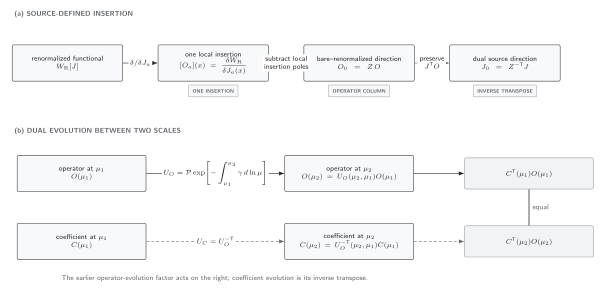
A source-defined insertion fixes $O_0=Z_OO$ and therefore $s_0=Z_O^{-\mathsf T}s$. Under scale evolution, $O(\mu_2)=U_OO(\mu_1)$ is compensated by $C(\mu_2)=U_O^{-\mathsf T}C(\mu_1)$, leaving $C^{\mathsf T}O$ unchanged. The original diagram is schematic and not to scale.

One-loop renormalization of a φ² insertion

Consider Euclidean scalar theory in $d=4-2\epsilon$,

$$\mathcal L = \frac12(\partial\phi)^2 +\frac12m^2\phi^2 +\frac{\lambda}{4!}\phi^4, \qquad O_0=\frac12\phi_0^2.$$

The insertion carries momentum $q$ into an amputated 1PI two-point vertex. Normalize the tree vertex to one. At order $\lambda$, the new graph has one quartic vertex and two propagators between that vertex and the insertion. Its scalar integral is

$$\begin{aligned} I(q^2;m^2) &= \mu^{2\epsilon} \int\frac{d^{4-2\epsilon}k}{(2\pi)^{4-2\epsilon}}\, \frac{1} {(k^2+m^2)\bigl[(k+q)^2+m^2\bigr]}\\ &= \frac1{16\pi^2} \left[ \frac1{\bar\epsilon} -\int_0^1dx\, \ln\frac{m^2+x(1-x)q^2}{\mu^2} \right] +\mathcal O(\epsilon), \end{aligned}$$

where

$$\frac1{\bar\epsilon} \equiv \frac1\epsilon-\gamma_E+\ln4\pi.$$

With the displayed Euclidean effective-action convention, the unrenormalized insertion vertex is

$$\Gamma_{O_0}^{(2)}(q) = 1-\frac{\lambda}{2}I(q^2;m^2) +\mathcal O(\lambda^2).$$

The pole is independent of $q$ and is therefore a local multiple of $O_0$. At this order $Z_\phi=1+\mathcal O(\lambda^2)$, so no external-field factor can cancel it. In the $\overline{\rm MS}$ convention,

$$O_0=Z_O[O]_{\overline{\rm MS}}, \qquad Z_O = 1-\frac{\lambda}{32\pi^2}\frac1{\bar\epsilon} +\mathcal O(\lambda^2).$$

Consequently,

$$\begin{aligned} \Gamma_{[O],\overline{\rm MS}}^{(2)}(q) &= Z_O^{-1}\Gamma_{O_0}^{(2)}(q)\\ &= 1+\frac{\lambda}{32\pi^2} \int_0^1dx\, \ln\frac{m^2+x(1-x)q^2}{\mu^2} +\mathcal O(\lambda^2), \end{aligned}$$

which is finite. This calculation isolates the new renormalization data: the ordinary theory already knew how to renormalize its propagator and coupling, but it did not yet specify the normalization of the local $\phi^2/2$ vertex.

There is a useful independent check. The operator conjugate to the renormalized mass is obtained by differentiating the bare action with respect to $m^2$ at fixed renormalized coupling. At one loop,

$$\frac{\partial\mathcal L_0}{\partial m^2} = \left( 1+\frac{\lambda}{32\pi^2}\frac1{\bar\epsilon} \right)\frac{\phi_0^2}{2} +\text{identity term} +\mathcal O(\lambda^2).$$

This is precisely $Z_O^{-1}O_0$ through the retained order. The equality is not an accident: differentiating a renormalized functional with respect to a parameter produces the finite insertion conjugate to that parameter, with vacuum terms included. It also explains why the insertion pole is tied to mass renormalization while remaining distinct from external-leg renormalization.

Finite normalization is part of the operator definition

Pole cancellation does not select a unique finite operator. A momentum-subtraction definition can require

$$\Gamma_{[O],{\rm MOM}}^{(2)}(q^2=Q_\star^2)=1.$$

Define

$$F(Q_\star^2) = \int_0^1dx\, \ln\frac{m^2+x(1-x)Q_\star^2}{\mu^2}.$$

Then the finite one-loop map is

$$[O]_{\rm MOM} = \left[ 1-\frac{\lambda}{32\pi^2}F(Q_\star^2) \right] [O]_{\overline{\rm MS}} +\mathcal O(\lambda^2).$$

The source transforms inversely so that $s[O]$ is unchanged. Neither operator normalization is more physical by itself. A matrix element or Wilson coefficient quoted without its operator scheme is incomplete; the invariant object is the consistently paired product.

The normalization condition must also say which matrix elements are used. An off-shell 1PI condition is convenient but gauge and kinematics dependent. An on-shell matrix element may eliminate equation-of-motion operators but can introduce infrared singularities. A symmetry Ward identity can fix a current normalization but only when the symmetry is nonanomalous and the regulator breaking has been restored. These are different definitions, not interchangeable shortcuts.

Vacuum subtraction and identity mixing

The zero-leg insertion already diverges in the free theory:

$$\left\langle O_0(x)\right\rangle = \frac12 \int\frac{d^dk}{(2\pi)^d}\frac1{k^2+m^2}.$$

Because $m^2\mathbf1$ has the same scalar quantum numbers and dimension as $\phi^2$, the closed local sector includes the identity with a dimensionful coefficient,

$$[O] = Z_O^{-1}O_0+c_{\mathbf1}m^2\mathbf1.$$

A condition such as $\langle[O]\rangle=0$ fixes $c_{\mathbf1}$, or the same term follows by differentiating the vacuum-energy counterterm. It does not affect connected matrix elements with external legs, which is why it can be missed in a two-point calculation. Omitting it nevertheless leaves the local operator undefined on the vacuum sector.

In massless dimensional regularization the tadpole is scaleless and may be set to zero. That is a statement about that regulator and kinematic limit, not a theorem forbidding identity mixing. A mass, curvature, boundary, cutoff, or other scale exposes the allowed local term again.

What one insertion fixes—and what it does not

Question	One-insertion answer	Additional data still needed
Are ordinary subdivergences removed?	Use the same action counterterms and forest recursion as the zero-source theory.	None, provided the ordinary renormalization scheme is declared.
Is the marked vertex finite?	Determine the linear source counterterms or $Z_O$ from insertion Green functions.	A finite operator normalization condition.
Is the operator sector closed?	Include every local operator allowed by power counting and exact quantum numbers, including identity or redundant directions when relevant.	Matrix closure tests, developed on the mixing page.
Are two insertions finite at coincidence?	Not implied by finite one-insertion vertices.	Source-quadratic counterterms and diagonal extensions on the contact-products page.
Is a matrix element observable?	Not by itself; it can depend on scheme, basis, gauge, and external states.	A consistently transformed coefficient or a symmetry-normalized physical observable.

Zimmermann’s normal-product construction gives an all-orders BPHZ definition of such local insertions and their mixing, rather than relying on a one-loop example Zimmermann 1973, pp. 536–569. The present page uses dimensional regularization and $\overline{\rm MS}$ because they make the pole and finite normalization map especially transparent.

Common pitfalls

Multiplying field renormalizations. Writing $[\phi^2]=Z_\phi^{-1}\phi_0^2$ accounts only for the two elementary factors. The marked vertex has divergent subgraphs of its own, and $Z_\phi$ begins too late to cancel the one-loop pole in the scalar example.

Calling normal ordering the interacting answer. Free normal ordering subtracts selected free contractions. Interactions generate new insertion subgraphs and operator mixing, so the renormalized composite operator depends on the interacting subtraction prescription.

Dropping the identity because external legs are present. Identity mixing is invisible in connected vertices with external fields but controls the vacuum insertion and parameter-derivative identities. State the sector on which the operator is meant to act.

Treating one-insertion finiteness as product finiteness. $[O](x)$ and $[O](y)$ can each be finite while their product diverges as $x\to y$. The missing information is local on the coincidence diagonal and belongs to higher powers of the source.

Exercises

1. Starting from $O_0=Z_OO$, derive the source relation required by $s_0^{\mathsf T}O_0=s^{\mathsf T}O$.

Solution

Substitution gives $s_0^{\mathsf T}Z_OO=s^{\mathsf T}O$ for every operator column $O$. Hence $s_0^{\mathsf T}Z_O=s^{\mathsf T}$ and

$$s_0=Z_O^{-\mathsf T}s.$$

Using $s_0=Z_O^{-1}s$ would work only in a one-dimensional or accidentally symmetric example; it is not the general dual transformation.

2. Reproduce the pole and finite term of the scalar bubble by introducing a Feynman parameter and shifting the loop momentum.

Solution

Use

$$\frac1{AB} = \int_0^1dx\, \frac1{\left[xA+(1-x)B\right]^2}$$

with $A=k^2+m^2$ and $B=(k+q)^2+m^2$. After shifting $\ell=k+(1-x)q$,

$$xA+(1-x)B = \ell^2+m^2+x(1-x)q^2.$$

The standard Euclidean integral gives

$$\mu^{2\epsilon} \int\frac{d^{4-2\epsilon}\ell}{(2\pi)^{4-2\epsilon}} \frac1{(\ell^2+\Delta)^2} = \frac1{16\pi^2} \left[ \frac1{\bar\epsilon}-\ln\frac{\Delta}{\mu^2} \right] +\mathcal O(\epsilon).$$

Integrating over $x$ yields $I(q^2;m^2)$. Multiplication by $-\lambda/2$ produces the pole $-\lambda/(32\pi^2\bar\epsilon)$, cancelled by $Z_O^{-1}-1$.

3. Explain why a condition on $\Gamma_{[O]}^{(2)}$ cannot fix identity mixing.

Solution

Functional differentiation of an identity insertion with respect to two elementary fields vanishes. Therefore $c_{\mathbf1}$ never appears in the two-leg 1PI vertex. A zero-leg condition, such as a vacuum expectation value or a derivative of the vacuum energy, is required.

Continue to Contact Terms and Renormalized Operator Products to renormalize two source derivatives at coincidence. Continue to Operator Mixing and Renormalization Matrices when more than one nontrivial local operator closes the one-insertion sector. For process-specific matrix elements, use Form Factors and Local Operator Insertions.

References

• Collins, John C. 1984; open-access reissue 2023. Renormalization: An Introduction to Renormalization, the Renormalization Group and the Operator-Product Expansion. Cambridge Monographs on Mathematical Physics. Cambridge University Press. DOI and Open PDF.

• Zimmermann, Wolfhart. 1973. “Composite Operators in the Perturbation Theory of Renormalizable Interactions.” Annals of Physics 77 (1–2): 536–569. DOI.