EFT Truncation Errors and Breakdown Diagnostics

An EFT truncation uncertainty estimates the contribution of operators and diagrams beyond a declared order; it is not a substitute for input, fit, regulator, or numerical uncertainty. A defensible estimate begins with an explicit expansion parameter and first omitted powers, states its coefficient and correlation assumptions, and is then tested against order-by-order calculations or withheld data. This page builds that workflow, applies it to the chapter’s heavy-mediator fixture, and gives stopping criteria for EFT breakdown.

Required background. Power Counting and Predictive Order defines the retained and first omitted orders. Loops, Counterterms, and Closure of an EFT Expansion explains why every retained order must include its counterterms and running.

A truncation model starts from the remainder

Write a dimensionless observable in a declared domain as

$$X(Q) = X_{\mathrm{ref}}(Q) \sum_{\nu\in\mathcal S}c_\nu(Q)q(Q)^\nu, \qquad q(Q)=\frac{Q}{\Lambda_b}<1,$$

where $\mathcal S$ is the set of powers allowed by the power counting. If the calculation retains the subset $\mathcal S_k$, its remainder is

$$\delta X_k(Q) = X_{\mathrm{ref}}(Q) \sum_{\nu\in\mathcal S\setminus\mathcal S_k} c_\nu(Q)q(Q)^\nu.$$

Let $p$ be the first omitted power. The familiar estimate

$$\delta X_k(Q) \sim X_{\mathrm{ref}}(Q)\,\bar c\,q(Q)^p$$

is conditional on three claims: the proposed $q$ describes the actual hierarchy, the normalization makes the omitted coefficients comparable to $\bar c$, and no unmodeled enhancement or singularity lies in the domain. It is an order estimate, not automatically a bound or a probability interval.

When all later allowed powers differ by $\Delta$ and one can justify the deterministic condition $|c_{p+j\Delta}|\leq\bar c$, the geometric tail gives the stronger conditional bound

$$|\delta X_k(Q)| \leq |X_{\mathrm{ref}}(Q)| \frac{\bar c\,q(Q)^p}{1-q(Q)^\Delta}.$$

Without the coefficient bound, the same expression is only a scale estimate. In an asymptotic expansion even that geometric tail need not apply, although the first omitted term can still estimate the error before optimal truncation.

Missing powers matter. A symmetry can remove an entire class of terms, while a kinematic cancellation can make one observable’s correction vanish accidentally. The first omitted power must come from the contribution inventory, not merely from the last nonzero difference that happened to be observed.

The order lattice below identifies the object being estimated. In the perturbative panel, the remainder begins with the first complete dashed column. In the shallow-scale panel, the leading resummation is already part of the retained prediction, so the uncertainty begins with the first omitted perturbative structure rather than with the next bubble in an infinite leading series.

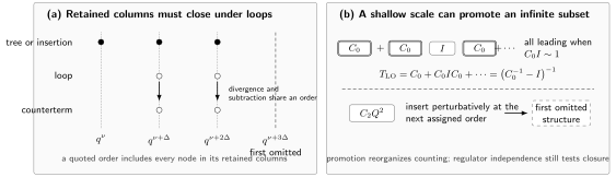
Predictive order requires closure. Panel (a) shows generic orders $q^\nu,q^{\nu+\Delta},\ldots$; each retained column must include every tree or insertion, loop, and local counterterm assigned to it, while the dashed column is the first omitted order. Panel (b) shows the distinct case $C_0I\sim1$, where a shallow scale promotes the entire $C_0$ iteration to leading order and higher-derivative structures remain perturbative. The diagram is schematic: $\Delta$ and the relative order of $C_2$ are theory dependent.

Learning a remainder from calculated orders

Suppose predictions are available at successive allowed orders. Their differences,

$$\Delta_\nu X(Q) = X_\nu(Q)-X_{\nu^-}(Q),$$

expose coefficient functions through

$$\widehat c_\nu(Q) = \frac{\Delta_\nu X(Q)} {X_{\mathrm{ref}}(Q)q(Q)^\nu}.$$

Here $\nu^-$ denotes the preceding calculated order, not necessarily $\nu-1$. A practical analysis plots these extracted coefficients over the full kinematic domain. Coefficients that remain comparable and vary on resolved physical scales support the proposed normalization. Systematic growth, rapid structure, or strong dependence on the fit window challenges it.

Several uncertainty statements can be built from this information, but their meanings differ.

• A leading-omitted-term estimate chooses $\bar c$ from calculated coefficients or mechanism-specific information and quotes $|X_{\mathrm{ref}}|\bar c q^p$. It is a transparent size rule, not a coverage statement.
• A deterministic interval requires explicit coefficient bounds or another theorem controlling the tail. Its validity is only as strong as those assumptions.
• A Bayesian credible interval assigns a probability model to coefficient sizes and, when needed, their correlations across energy, angle, and observables. Calculated orders update the model; the resulting degree-of-belief interval must identify its prior and conditioning data.
• A frequentist interval needs a repeated-sampling construction and an ensemble under which coverage is defined. Calling a heuristic band “$68\%$” does not create that ensemble.

Naturalness priors and order-by-order coefficient information were developed into Bayesian EFT truncation models by Furnstahl et al. 2015, §§ II–IV. Because the same omitted coefficients usually affect many kinematic points, treating pointwise theory errors as independent can grossly overstate the information in a fit. Gaussian-process models provide one conditional way to represent those correlations and test the assumed coefficient functions Melendez et al. 2019, §§ II–IV.

No statistical construction repairs an incomplete retained order. A missing same-order loop or counterterm is a calculation error, not a random higher-order effect.

Synthetic heavy-mediator breakdown test

Use the fixed-angle scalar fixture from Effective Field Theory as a Controlled Expansion. Normalize the exact amplitude to its leading term,

$$X_{\mathrm{exact}}(q) = \frac13 \left[ \frac{1}{1-q^2} +\frac{1}{1+q^2/3} +\frac{1}{1+2q^2/3} \right], \qquad q=\frac{E}{M}.$$

Its local expansion is

$$X_{\mathrm{exact}}(q) = 1 +\frac{14}{27}q^4 +\frac29q^6 +\frac{98}{243}q^8 +\cdots.$$

The $q^2$ coefficient vanishes because $s+t+u=0$; it would be wrong to infer from this zero that the next uncertainty begins at $q^8$. Truncating through $q^4$ gives

$$X_4(q)=1+\frac{14}{27}q^4, \qquad R_4(q)=X_{\mathrm{exact}}(q)-X_4(q).$$

Generate synthetic exact values with a hidden $M_{\mathrm{true}}=1\,\mathrm{TeV}$. The last two columns test the first-omitted-term form. The effective coefficient is $c_{\mathrm{eff}}=R_4/q^6$, and, using the known leading coefficient $c_6=2/9$, a pointwise scale estimator is

$$\widehat M(E) = E\left(\frac{2/9}{R_4(E)}\right)^{1/6}.$$

$E$ (GeV)	$q$	$X_{\mathrm{exact}}$	$R_4$	$c_{\mathrm{eff}}$	$\widehat M/M_{\mathrm{true}}$
100	0.1	1.000052078	$2.263\times10^{-7}$	0.226	0.997
200	0.2	1.000844915	$1.529\times10^{-5}$	0.239	0.988
300	0.3	1.004390371	$1.904\times10^{-4}$	0.261	0.973
400	0.4	1.014485912	$1.212\times10^{-3}$	0.296	0.953
500	0.5	1.037851038	$5.444\times10^{-3}$	0.348	0.928

At the two lowest energies, where $q^8$ and higher terms are smallest, the inferred scale is within about one percent of the true pole scale. A log–log fit of $R_4$ against $E$ through $400\,\mathrm{GeV}$ gives slope $6.18$, close to the predicted six but already shifted by higher powers. The rising $c_{\mathrm{eff}}$ and downward drift of $\widehat M$ at larger $E$ are not statistical fluctuations: they resolve the $q^8$ and higher terms.

For a deliberately conservative band, assume all coefficients from $q^6$ onward have magnitude at most $\bar c=1$. Since only even powers occur, the conditional tail bound is

$$B_4(q)=\frac{q^6}{1-q^2}.$$

It contains the exact residual at every tabulated point; at $q=0.5$, $B_4=2.08\times10^{-2}$ while $R_4=5.44\times10^{-3}$. This successful synthetic coverage validates the band only for this fixture and domain. It does not prove that $\bar c=1$ or the geometric tail applies in another EFT.

There is also an identifiability limit. If $c_6$ is unknown, low-energy residuals determine the combination $c_6/M^6$, not $c_6$ and $M$ separately. Inferring a breakdown-scale distribution therefore requires matching information, multiple calculated orders, a coefficient prior, or additional observables. A sharp numerical value for $\Lambda_b$ without one of those inputs is overinterpreted.

A reproducible calculation lets the expansion parameter, retained order, and coefficient assumptions vary so that this residual-scaling test can be repeated rather than accepted from a single table.

Separating truncation, parameter, and numerical errors

For data vector $d$ and prediction $X_k(\theta)$, a useful bookkeeping form is

$$d = X_k(\theta) +\delta_{\mathrm{EFT}} +\delta_{\mathrm{num}} +\epsilon_{\mathrm{data}}.$$

The terms have different origins and diagnostics.

EFT truncation. This changes predictably with EFT order and kinematics. Its correlations arise because common omitted coefficients feed multiple points and observables. It should shrink by the declared powers when the order is raised.

Input and fit uncertainty. Experimental covariance and uncertain external inputs propagate through the fitted parameters. For a parameter covariance $C_\theta$, linear propagation gives $J C_\theta J^T$ with $J_{i\alpha}=\partial X_i/\partial\theta_\alpha$. If $C_\theta$ was itself inferred from the same data, adding both covariances naively can double count information; a joint likelihood or posterior is safer.

Numerical uncertainty. This is measured by changing integration tolerances, basis size, lattice spacing, solver precision, or Monte Carlo statistics. It must be driven parametrically below the claimed EFT uncertainty. Repeating a calculation at higher EFT order while leaving an equally large discretization error does not test EFT convergence.

For scale, imagine the synthetic values above were reported with independent data uncertainty $2\times10^{-4}$ and verified numerical error below $10^{-6}$. At $100\,\mathrm{GeV}$ the true EFT residual is hidden beneath both the data error and the chosen numerical target; at $300\,\mathrm{GeV}$ it is comparable to the data error; at $400\,\mathrm{GeV}$ it dominates. Those regimes should not be compressed into one energy-independent percentage.

Independent covariance components may be added only after independence is justified. Regulator and renormalization-scale variation are diagnostics of missing contributions, not automatically independent random draws to add in quadrature with the truncation model.

Validation and breakdown diagnostics

A proposed error model should pass tests that were not used merely to tune its width.

1. Residual scaling. Compare with exact or withheld data and examine $R_k/[X_{\mathrm{ref}}q^p]$. A stable order-one pattern supports the first omitted power; systematic growth or a wrong log–log slope does not.
2. Order-by-order calibration. Use lower orders to predict the next calculated order, then check interval coverage and coefficient distributions. Refit hyperparameters without using the order being tested.
3. Fit-window stability. Raise the maximum fitted energy or momentum. Wilson coefficients and inferred $\Lambda_b$ should remain compatible until the tested domain approaches breakdown.
4. Correlated checks. Whiten residuals using the proposed covariance and inspect energy, angle, and observable dependence. Pointwise coverage can look acceptable while coherent residual structure reveals a failed correlation model.
5. Auxiliary-choice checks. Vary regulators, bases, schemes, and numerical controls over admissible ranges. Dependence at or below the retained order signals missing renormalization or inconsistent implementation.

Breakdown is indicated by converging evidence rather than a universal numerical cutoff: $q$ approaches unity; a new pole, threshold, or nonanalyticity enters; extracted coefficients grow or acquire unresolved structure; fit results drift; successive orders stop improving; or withheld-data coverage fails coherently. Inflating the truncation band until every point is covered hides, rather than diagnoses, such failure. The correct response can be a smaller domain, a different counting, a promoted interaction, or new explicit degrees of freedom.

As of August 2026, published uncertainty frameworks remain conditional on their coefficient, correlation, and domain assumptions. Correlated Gaussian-process diagnostics can infer expansion parameters and breakdown scales, but an application to nucleon–nucleon potentials found that stationarity across energy and angle was not generally satisfied Millican et al. 2024, §§ II–IV. In collider SMEFT, the LHC EFT Working Group documented multiple proposals without adopting a universal prescription Brivio et al. 2022, pp. 1–3, 32–35, arXiv PDF. A recent nuisance-parameter construction uses the calculable dimension-six-squared contribution to model missing $\Lambda^{-4}$ effects in specified SMEFT signal-rate examples; it is a proposal for that setting, not a general theorem about EFT errors Assi, Martin, and Shepherd 2026, §§ 2–4, arXiv PDF.

A common uncertainty and validation checklist

The same record used on the preceding pages keeps the truncation model adjacent to the other uncertainties and to explicit failure triggers.

Component	Record explicitly	Diagnostic or failure trigger
Domain and expansion parameters	Observable, kinematic window, $q_i(Q)$, hard scales, thresholds, and correlations among small parameters	A threshold enters, some $q_i\not\ll1$, or the assumed relation among parameters fails
Retained order and inventory	Highest order $k$, every tree, loop, insertion, counterterm, and parameter correction included	An omitted contribution has the same assigned order as a retained one
Coefficient assumptions	Operator normalization, scheme and scale, expected coefficient sizes, symmetry suppressions, and any priors	Coefficients drift with fit window or require unexplained enhancement
EFT truncation	First omitted powers, reference size, correlation model across energies and observables, and interval interpretation	Residuals do not scale with the predicted powers or coverage fails on withheld data
Input and fit uncertainty	Experimental or synthetic inputs, covariance, fitted combinations, and propagation method	Results are unstable under admissible input or fit-window changes
Numerical uncertainty	Solver, discretization, integration, rounding, convergence tolerance, and reproducibility data	Numerical changes are not parametrically below the claimed EFT error
Matching and running	Matching order and scale, anomalous dimensions, threshold sequence, and residual $\mu$ dependence	Scale cancellation fails through the retained order or a threshold is double counted
Regulator, basis, and scheme checks	Regulator range, required counterterms, field/basis map, and scheme transformation	Predictions depend on an auxiliary choice at or below the claimed order
Model discrepancy and breakdown	Effects not represented by the EFT, validation observables, stopping rule, and alternative field content	Persistent structured residuals, new nonanalyticity, or failure across observables

Common pitfalls

The last visible correction is the error bar. An accidental zero or unusually small coefficient can make the last shift misleading. Use the first omitted contribution set and test the coefficient assumptions across orders and observables.

Every kinematic point has an independent theory error. Common Wilson coefficients induce correlated shifts. Ignoring those correlations can make a dense grid look more informative than it is.

The regulator or fit cutoff is the breakdown scale. A regulator is an auxiliary calculation choice and a fit cutoff is an analysis decision. The breakdown scale is tied to the physical analytic structure and the tested convergence pattern.

A wider band restores validity. A band can express uncertainty inside a modeled domain. It cannot turn a resolved threshold or failed field content into a valid EFT description.

Exercises

For the heavy-mediator fixture at $q=0.3$, evaluate the conditional band $B_4=q^6/(1-q^2)$ and compare it with the exact residual in the table.

Solution

The band is

$$B_4(0.3) = \frac{0.3^6}{1-0.3^2} = 8.01\times10^{-4}.$$

The exact residual is $1.904\times10^{-4}$, about $24\%$ of the band. The check confirms coverage for this point under the stated coefficient bound; it does not assign a probability to the interval.

Suppose a residual fit at low energy determines $R_4(E)=A E^6$. Show why it cannot determine both $c_6$ and $\Lambda_b$ without additional information.

Solution

The leading remainder model is

$$R_4(E) = c_6\left(\frac{E}{\Lambda_b}\right)^6,$$

so the fitted coefficient is $A=c_6/\Lambda_b^6$. For any positive rescaling $c_6\to\alpha^6c_6$ and $\Lambda_b\to\alpha\Lambda_b$, $A$ is unchanged. Matching information, a prior on $c_6$, another known order, or additional observables are needed to break the degeneracy.

References

• Assi, Benoît, Adam Martin, and William Shepherd. “EFT Validity and Truncation Uncertainty from Few Nuisance Parameters.” arXiv:2607.02649 [hep-ph] (2026). arXiv
• Brivio, Ilaria, et al. “Truncation, Validity, Uncertainties.” CERN-LHCEFTWG-2021-002 and CERN-LPCC-2022-01, arXiv:2201.04974 [hep-ph] (2022). arXiv
• Furnstahl, R. J., N. Klco, D. R. Phillips, and S. Wesolowski. “Quantifying Truncation Errors in Effective Field Theory.” Physical Review C 92 (2015): 024005. DOI
• Melendez, J. A., R. J. Furnstahl, D. R. Phillips, M. T. Pratola, and S. Wesolowski. “Quantifying Correlated Truncation Errors in Effective Field Theory.” Physical Review C 100 (2019): 044001. DOI
• Millican, P. J., R. J. Furnstahl, J. A. Melendez, D. R. Phillips, and M. T. Pratola. “Assessing Correlated Truncation Errors in Modern Nucleon–Nucleon Potentials.” Physical Review C 110 (2024): 044002. DOI