

Renormalized Perturbation Theory and Counterterm Rules
Renormalized perturbation theory is ordinary perturbation theory with a disciplined split of the regulated action. One part contains finite renormalized fields and parameters; the other contains local counterterm vertices whose coefficients are expanded in loop order. At any declared order, genuine loop graphs, lower-loop graphs with counterterm insertions, and the counterterm of that order must all be included.
The split itself is not physical. Bare quantities depend on the regulator, renormalized parameters depend on their defining scheme and scale, and counterterms depend on both. The meaningful output is a finite Green function or amplitude expressed in terms of fixed renormalized inputs, followed—when appropriate—by external-state reduction and comparison with a non-input observable.
Required background. The R-Operation, Forest Formula, and Overlapping Divergences explains why lower-order counterterm insertions are required in higher-loop graphs. Dimensional Regularization and Minimal Subtraction fixes , the modified-MS scale convention, and the separation of ultraviolet from infrared poles.
Helpful background. UV/IR Poles and the Renormalized-Amplitude Interface supplies the regulated loop-amplitude interface consumed here; loop reduction and integral evaluation remain in Volume 4.
The bare action becomes a finite action plus local vertices
Section titled “The bare action becomes a finite action plus local vertices”For a precise scalar example, Wick rotate the globally defined Minkowski theory and use the Euclidean bare action
Define the renormalized field and the post-substitution additive counterterm coefficients by
The factors of in the last line matter. If one instead defines multiplicative constants for and , their products with must be expanded before reading off vertices. With the definitions above,
where
This equality is an algebraic reparametrization of the regulated theory. It is not an approximation and does not say that the bare and counterterm pieces are separately observable. Collins shows how the local graph counterterms generated by the forest formula assemble with the correct symmetry factors into counterterm terms in the action Collins 1984/2023, §§ 5.6–5.7, pp. 112–125.
For the Euclidean expansion of , the elementary rules are:
| Element | Momentum-space rule | Perturbative role |
|---|---|---|
| Renormalized propagator | Used on ordinary internal lines | |
| Renormalized quartic vertex | Ordinary interaction vertex | |
| Two-point counterterm vertex | Cancels local kinetic and mass terms | |
| Four-point counterterm vertex | Cancels the local quartic term and implements its finite condition |
The minus signs in this table come from expanding . In a 1PI effective-action coefficient, the corresponding terms appear with the signs written in . Stating which convention is being used prevents the common mistake of importing a Minkowski vertex sign into a Euclidean inverse Green function.
Loop order is carried by counterterm coefficients
Section titled “Loop order is carried by counterterm coefficients”Introduce an explicit bookkeeping parameter :
A graph with ordinary loops and counterterm vertices labelled by loop orders contributes at
Thus “one loop” means more than “draw graphs with one loop.” At total order one, include one-loop graphs built from renormalized vertices and tree graphs with a first-order counterterm. At total order two, include:
- genuine two-loop graphs;
- one-loop graphs with one first-order counterterm insertion;
- tree contributions from second-order counterterms;
- any allowed tree topology with counterterm orders summing to two;
- the order-two expansion of external residues, parameter conversions, and lower-order expressions when computing an S-matrix element or derived observable.
This is the action-level version of the forest formula. A lower-order counterterm insertion removes a subdivergence; the new counterterm at the current order removes the remaining overall local divergence. Counterterms are not resummed into the free propagator unless a separate reorganization has been declared, because doing so silently mixes perturbative orders.
One-loop scalar two-point rule
Section titled “One-loop scalar two-point rule”In the -invariant scalar theory, the only one-loop 1PI two-point graph is the tadpole. It is independent of the external momentum, so it can require a mass counterterm but not a field-strength counterterm. Define
Analytic continuation gives
where
The loop contribution to the Euclidean 1PI two-point coefficient is . Modified minimal subtraction therefore gives
The pole cancels in the sum, leaving
There is no one-loop term in this theory, hence no one-loop residue renormalization. That is a property of this example, not a general rule: derivative interactions, gauge theories, Yukawa theories, and scalar theory at two loops do renormalize the field.
One-loop scalar four-point rule
Section titled “One-loop scalar four-point rule”Take all external Euclidean momenta incoming, . In this section denotes the dimensionless coefficient after the common factor has been removed. The remaining one-loop integral therefore carries one factor of . Define
The logarithmic bubble in channel is
Each bubble has symmetry factor . The three channels give the pole
Consequently,
and the finite modified-MS four-point coefficient is
The pole is local and momentum independent; the channel logarithms remain. After analytic continuation they carry the physical cuts. A momentum-dependent counterterm chosen to remove those logarithms would be nonlocal and would change the theory rather than renormalize it.
The factors above use . If one instead writes , the pole coefficients expressed with that differ by a factor of two. The four-dimensional beta function does not: the compensating engineering term changes from to . Never compare pole coefficients until the dimensional convention and coupling normalization have been aligned.
From graph rules to a finite prediction
Section titled “From graph rules to a finite prediction”The scalar example stops at renormalized 1PI functions. A scattering prediction also requires pole residues and analytic continuation. Calculations A and B in the map impose the same finite input and field-normalization conditions before comparing a quantity not used as an input.
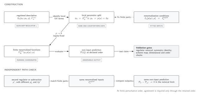
The two branches calculate the same renormalized quantity through a declared order, using different bare data. can be a fixed-normalization Green function; it becomes a physical observable only after the required state or operator normalization and continuation. Regulator artifacts and omitted perturbative terms are distinct. The schematic map is not a nonperturbative existence proof.
For the worked scalar rules, the common regulator-comparison fields specialize as follows:
| Checkpoint | Declared entry | Required test |
|---|---|---|
| Regulator | Dimensional regularization, | Keep ultraviolet and any infrared poles separately labelled |
| Subtraction | Modified minimal subtraction with the stated convention | Remove only the prescribed local pole terms |
| Symmetry | Euclidean rotations and | No odd-field counterterm; two- and four-point tensors have the allowed form |
| Renormalized coordinates | and | Tie them to two finite input conditions before calling another quantity a prediction |
| Order-one insertions | , , | Every pole in and cancels |
| Finite structure | Tadpole constant and three channel logarithms | Preserve nonlocal momentum dependence and crossing symmetry |
| Removal limit | at fixed renormalized inputs | Finite result with no residual |
| Residual dependence | and scheme dependence at finite order | Cancel against running and finite parameter maps to the calculated accuracy |
This record is not a proof that a chosen observable is correct. It is the minimum information needed to reproduce what was renormalized and to distinguish a missing counterterm from a convention mismatch.
General assembly rule
Section titled “General assembly rule”For a renormalized -point 1PI function through total loop order , use
where is the sum of every graph satisfying
A reproducible calculation should record, for each term:
- graph topology and symmetry factor;
- ordinary loop count;
- every counterterm vertex and the order assigned to it;
- regulator and subtraction convention;
- ultraviolet and infrared pole labels;
- finite renormalization conditions;
- external-field or operator renormalization;
- the truncation remainder.
For an S-matrix element, append the external pole residues and express masses and couplings in the declared input scheme. For a composite insertion, include operator mixing. For gauge theories, solve the symmetry identities for the complete counterterm action rather than renormalizing each vertex independently. For EFTs, include every operator that enters at the working power-counting order, even if its canonical dimension is high.
Common pitfalls
Section titled “Common pitfalls”Calling a loop graph the complete loop order. A one-loop graph is only one contribution at order one. The first-order counterterm graph is required for finiteness.
Reading additive counterterms before field substitution. If , the mass and coupling coefficients acquire factors of and . Define the post-substitution coefficients or expand the products consistently.
Using counterterms inside the free propagator without declaring a reorganization. Resumming them mixes infinitely many nominal orders. Keep counterterms as insertions in ordinary fixed-order perturbation theory.
Comparing and pole residues directly. The symbols denote different distances from four dimensions. Translate both the pole and the engineering part of the beta function.
Removing finite channel logarithms. They are not arbitrary ultraviolet terms. They encode kinematics and, after continuation, physical thresholds.
Calling or an observable. They are scheme-dependent coordinates. A physical input defines them, and a separate non-input quantity tests the calculation.
Exercises
Section titled “Exercises”1. One-loop field strength. Why is in the worked scalar theory?
Solution
The only one-loop 1PI two-point graph is a tadpole. It has no dependence on the external momentum, so its local divergence is proportional to , not . A kinetic counterterm first appears at higher loop order in this model.
2. Four-point coefficient. Recover the total pole factor from the channel bubbles.
Solution
There are three crossing channels, and each pair of quartic vertices joined into a one-loop bubble has symmetry factor . Thus the loop sum is in its pole part, giving .
3. Two-loop inventory. A two-loop two-point graph contains a one-loop divergent four-point subgraph. Which term removes that subdivergence?
Solution
The required term is a one-loop graph with the first-order quartic counterterm inserted in place of the divergent subgraph. A second-order two-point counterterm then removes the remaining overall local divergence.
Finite rule set
Section titled “Finite rule set”The operational statement is
Once every term at the requested order is present, local poles cancel and the remaining momentum dependence is finite and dynamical. The counterterm coefficients then become the inputs to symmetry identities, finite scheme maps, and renormalization-group equations.
Continue to Symmetry Constraints and the Space of Counterterms to learn which apparently local coefficients are related or forbidden. Continue to Renormalization Conditions, Schemes, and Finite Parts to replace modified-MS coordinates by on-shell or momentum-subtraction ones. Use Regulator Removal and Renormalized Predictions for the chapter-level prediction test.
References
Section titled “References”- Collins, John C. 1984; open-access reissue 2023. Renormalization: An Introduction to Renormalization, the Renormalization Group and the Operator-Product Expansion. Cambridge Monographs on Mathematical Physics. Cambridge University Press. DOI and Open PDF.
Original QFT.org content:CC BY 4.0, unless an item supplies different terms. Third-party material retains its own terms.