Power Counting of Divergences and Perturbative Renormalizability

Power counting predicts which ultraviolet divergences can occur by scaling all independent loop momenta to infinity. The superficial degree of a full graph is only the first pass: the same test must be applied to every proper subgraph, and the resulting local structures must be filtered by Lorentz symmetry, internal symmetries, statistics, and any Ward or Slavnov–Taylor identities. The output is a counterterm inventory, not a value for the graph.

The classification “perturbatively renormalizable” means that this inventory closes on a finite set of interaction types order by order. It does not prove ultraviolet completeness. Conversely, a coupling of negative mass dimension does not make a theory unpredictive: in an EFT, only finitely many operators contribute at a fixed order in the declared expansion.

Required background. Ultraviolet Sensitivity and the Renormalization Problem explains why the remaining ambiguity is local, while Diagrammatics and Symmetry Factors supplies loop, line, vertex, and subgraph bookkeeping.

Helpful background. Anatomy of a Loop Integral is useful for identifying independent loop momenta and numerator powers before the degree count.

Superficial degree from graph topology

Let $G$ be a connected graph in $d$ spacetime dimensions. Suppose a propagator of species $a$ falls as $k^{-r_a}$ at large Euclidean momentum and a vertex of type $v$ carries $N_v^{(\partial)}$ powers of momentum. If $L$ is the number of independent loops, $I_a$ the number of internal lines of species $a$ , and $V_v$ the number of vertices of type $v$ , the superficial ultraviolet degree is

\omega(G) =dL -\sum_a r_a I_a +\sum_v N_v^{(\partial)}V_v.

The name superficial is literal. This count scales all loop momenta together and ignores cancellations caused by symmetric integration, gauge identities, special kinematics, or numerator algebra. It also says nothing about a region in which only the momenta of a proper subgraph become large.

For ordinary relativistic scalar, gauge, and ghost propagators $r=2$ ; for a Dirac propagator $r=1$ . Higher-derivative kinetic terms, nonrelativistic propagators, anisotropic scaling, or resummed propagators require a new count from their actual asymptotic behavior.

For a connected graph,

L=I-V+1,

where $I=\sum_a I_a$ and $V=\sum_v V_v$ . Line-end counting for species $a$ gives

\sum_v n_{av}V_v=2I_a+E_a,

with $n_{av}$ the number of fields of species $a$ at vertex $v$ and $E_a$ the number of external legs. For canonical relativistic kinetic terms, these identities turn the degree into

\boxed{ \omega(G) =d -\sum_a E_a[\Phi_a] -\sum_v V_v[g_v] }

where $[\Phi_a]$ is the canonical field dimension and

[g_v] =d-N_v^{(\partial)} -\sum_a n_{av}[\Phi_a]

is the canonical dimension of the vertex coefficient. The boxed formula is a diagnostic for the stated propagators and vertices. It is not a substitute for checking subgraphs or symmetry.

Four-dimensional scalar quartic theory

For

\mathcal L =\frac12(\partial\phi)^2 -\frac12m^2\phi^2 -\frac{\lambda}{4!}\phi^4

in $d=4$ , $[\phi]=1$ and $[\lambda]=0$ . A connected graph containing quartic vertices therefore has

\omega(G)=4-E.

The same result follows directly:

4V=2I+E, \qquad L=I-V+1, \qquad 4L-2I=4-E.

The candidate counterterms follow from the external-leg count and the polynomial degree allowed by $\omega$ .

External legs	Superficial degree	Local structures before symmetry and redundancies	$\mathbb Z_2$ -invariant scalar result
$E=0$	$4$	vacuum terms with no external fields	vacuum-energy counterterm
$E=2$	$2$	$\phi^2$ and two-derivative two-field terms	mass and kinetic counterterms
$E=4$	$0$	four-field term with no derivatives	quartic counterterm
odd $E$	varies	odd-field monomials	forbidden by $\phi\mapsto-\phi$
$E\ge6$	$<0$	none from the overall graph	superficially convergent, but subdivergences may remain

This table is deliberately an upper bound. A particular $E=2$ graph need not contain both a mass and a wavefunction divergence at every loop order. For example, the one-loop quartic tadpole is momentum independent, so it can renormalize the mass but not the kinetic term. Power counting says a $p^2$ divergence is allowed somewhere in the two-point sector; it does not promise that every graph realizes the maximum degree.

Every ultraviolet subgraph must pass the same test

A graph with $\omega(G)<0$ can still diverge. Hold its external momenta fixed and scale only the loop momenta belonging to a proper subgraph $\gamma$ . If

\omega(\gamma)\ge0,

that region contains a subdivergence. Contracting $\gamma$ to a point identifies the local vertex that its counterterm inserts into the reduced graph $G/\gamma$ .

In the massive Euclidean setting with generic external momenta, Weinberg’s convergence criterion requires negative ultraviolet degree for the graph and all relevant subgraphs after the prescribed subtractions. Its hypotheses matter: exceptional or massless kinematics can add infrared singular regions, and cancellations visible only after summing graphs require the corresponding symmetry argument Weinberg 1960, pp. 838–849.

Subgraphs can be related in three ways. The distinction controls which subtractions can be applied simultaneously, as the diagram shows.

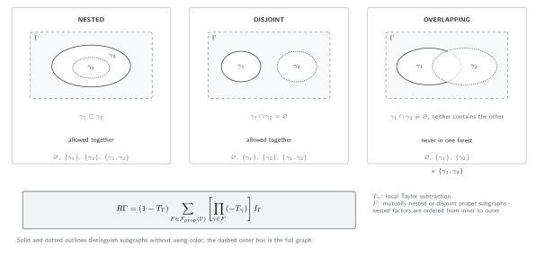
Nested and disjoint divergent subgraphs can occur together in one forest, whereas two overlapping subgraphs must occur in separate forest terms; a final local Taylor subtraction removes the overall divergence. — Compatibility of ultraviolet subgraphs. Nested and disjoint proper subgraphs may be members of the same forest; overlapping subgraphs are each subtracted, but never as a simultaneous pair. The displayed forest formula is schematic: $T_\gamma$ extracts the allowed local Taylor polynomial, nested operations are ordered from inner to outer, and the full graph receives the final overall subtraction. The set diagram is not a particular Feynman graph and is not to scale.

The same content can be read without the image:

Relation between $\gamma_1$ and $\gamma_2$	May both occur in one forest?	Reason
Nested, $\gamma_1\subset\gamma_2$	Yes	The inner divergence is removed before the outer subgraph is replaced by its local part
Disjoint, $\gamma_1\cap\gamma_2=\varnothing$	Yes	Their loop variables and local contractions can be treated independently
Overlapping, nonempty intersection with neither contained in the other	No	Simultaneous contraction would double assign shared lines; separate forest terms handle the two regions

This page uses the forest only to expose the diagnostic. Local Counterterms and Subdivergence Structure explains why the extracted terms are local, and The R-Operation, Forest Formula, and Overlapping Divergences develops the recursive construction and its detailed combinatorics. Zimmermann’s formula supplies the systematic solution to that recursion Zimmermann 1969, pp. 208–234.

Symmetry filters the power-counting list

Power counting lists local tensors with allowed dimension and field content. The theory’s symmetries then select the admissible combinations.

For a real scalar with $\mathbb Z_2$ symmetry, odd powers of $\phi$ are excluded. Lorentz invariance contracts derivative indices, and integration by parts can relate apparently different monomials. For fermions, statistics and internal representations constrain index contractions. In a gauge theory, a term-by-term list built only from canonical dimensions is insufficient: the counterterm functional must satisfy the appropriate Ward or Slavnov–Taylor identity, possibly after allowed restoration of a regulator-induced breaking.

Symmetry can improve an individual amplitude beyond its naive degree. It cannot be invoked as an unexplained cancellation. A sound counterterm inventory records

the field content and representations;
the maximum local dimension or EFT order;
Lorentz and internal singlet conditions;
discrete symmetries and ghost number where relevant;
integration-by-parts and equation-of-motion qualifications; and
the functional identity that relates coefficients.

The detailed identity analysis belongs to Symmetry Constraints and the Space of Counterterms. At the power-counting stage, the safe procedure is to retain every structure not demonstrably forbidden.

Relevant, marginal, and irrelevant couplings

Canonical dimensions give a useful perturbative classification near the Gaussian fixed point.

Coefficient dimension	Traditional name	Effect of more insertions on $\omega$	Perturbative implication
$[g_v]>0$	superrenormalizable interaction	lowers $\omega$	only a bounded set of graph topologies or orders can diverge
$[g_v]=0$	power-counting-renormalizable interaction	leaves $\omega$ unchanged	the counterterm types can close on a finite set
$[g_v]<0$	power-counting-nonrenormalizable interaction	raises $\omega$	increasing insertions require operators of increasing dimension

The words relevant, marginal, and irrelevant become full RG statements only after a fixed point and flow direction are specified. Here they refer to Gaussian canonical counting. Anomalous dimensions can change the classification at an interacting fixed point.

Consider adding $c_6\phi^6/\Lambda^2$ in four dimensions. Its coefficient has dimension $-2$ , and each insertion contributes $+2$ to the superficial degree:

\omega(G)=4-E+2V_6

for a graph whose other interactions have dimensionless coefficients. Across arbitrarily many $V_6$ , no finite list of counterterm dimensions closes. But an EFT calculation truncated at a fixed power of $1/\Lambda$ permits only a bounded number of such insertions and therefore requires only a finite operator basis at that order. “Nonrenormalizable” in the old all-orders sense is compatible with systematic low-energy prediction.

The converse warning is equally important. A finite counterterm list near the Gaussian point does not show that the theory can be continued to arbitrarily high energy. Landau singularities, vacuum instability, nonperturbative obstructions, or the absence of a suitable ultraviolet fixed point are separate questions.

A reproducible degree-counting workflow

For each graph or declared interaction set:

State the asymptotic scaling. Record $d$ , the propagator falloffs, derivative numerators, and whether the scaling is relativistic or anisotropic.
Count the full graph. Determine $L$ , $I_a$ , $V_v$ , and $E_a$ ; compute $\omega(G)$ in two ways when possible.
Enumerate proper candidate subgraphs. Include every connected 1PI subgraph with the field content of an allowed local vertex; do not inspect only visually obvious loops.
Compute each $\omega(\gamma)$ . Record nested, disjoint, and overlapping relations among subgraphs.
Translate degree into local tensors. A degree $r$ allows a momentum polynomial through degree $r$ , subject to parity and index structure.
Apply symmetry and redundancy filters. State each identity or equivalence used to remove or relate a candidate.
Classify the interaction set. Specify whether the claim is all-order perturbative closure or finite-order EFT closure.
Hand off correctly. Forest recursion performs the subtraction; loop-integration machinery evaluates the regulated terms; neither is replaced by the degree count.

Dimensional analysis checks the result. A counterterm coefficient multiplying an operator $\mathcal O_i$ of dimension $\Delta_i$ must have dimension $d-\Delta_i$ . If the graph result cannot supply that dimension from masses, external momenta, and the regulator or subtraction scale, the proposed structure is inconsistent.

Common pitfalls

Checking only the full graph. A six-point graph in four-dimensional $\phi^4$ theory has $\omega=-2$ , yet it may contain a two- or four-point divergent subgraph. List and count every proper 1PI candidate.

Treating $\omega\ge0$ as proof of a divergence. The degree is an upper bound. Odd integrands, tensor contractions, or symmetry identities can cancel the leading term; demonstrate the cancellation rather than building it into the initial count.

Using canonical dimension as complete EFT power counting. Low-energy kinematics, symmetry breaking, loops, small couplings, and promoted nonperturbative interactions can reorder operators. Canonical dimension is an input to a counting rule, not always the rule itself.

Calling power-counting renormalizability ultraviolet completion. Closure of perturbative counterterms says nothing by itself about the existence of the theory at arbitrarily short distance.

Ignoring infrared regions. Negative ultraviolet degrees do not exclude soft or collinear singularities. In a scaleless dimensional integral, ultraviolet and infrared poles can cancel in the total zero; label their origins separately.

Exercises

1. Derive the scalar result. For a connected four-dimensional $\phi^4$ graph, use $4V=2I+E$ and $L=I-V+1$ to derive $\omega=4-E$ .

Solution

The loop measure and scalar propagators give $\omega=4L-2I$ . Substitute $L=I-V+1$ to obtain $\omega=2I-4V+4$ . The line-end identity gives $2I=4V-E$ , hence $\omega=4-E$ .

2. Find the hidden subdivergence. A connected six-point $\phi^4$ graph contains a one-loop four-point subgraph. Classify the full graph and the subgraph.

Solution

The full graph has $E=6$ and $\omega(G)=-2$ , so it is superficially convergent. The four-point subgraph has $\omega(\gamma)=0$ and can be logarithmically divergent. Its local quartic counterterm must be inserted before the convergence of the reduced graph is assessed.

3. Classify an EFT insertion. In $d=4$ , a scalar operator $(\partial_\mu\phi\partial^\mu\phi)\phi^2/\Lambda^2$ has four fields and two derivatives. Find the coefficient dimension and explain why a fixed $1/\Lambda^2$ calculation still needs finitely many counterterms.

Solution

The operator dimension is $4[\phi]+2=6$ , so its coefficient has dimension $-2$ . It is power-counting nonrenormalizable in an all-orders expansion with arbitrarily many insertions. At order $1/\Lambda^2$ , however, only one insertion is permitted; the degree and symmetries then allow only a finite set of dimension-six and lower counterterms needed for closure at that order.

What the diagnostic establishes

Power counting answers two bounded questions: which ultraviolet regions require attention, and which local operator classes can absorb them. It does not perform the subtraction, calculate a coefficient, or prove a continuum limit. The complete diagnostic is

\text{full-graph degree} + \text{subgraph degrees} + \text{symmetry filter} + \text{declared order}.

Continue to QFT Regulator Families and Their Tradeoffs to choose a regulator consistent with the desired identities. Continue to Local Counterterms and Subdivergence Structure when the next question is why the subtraction is local, or to The R-Operation, Forest Formula, and Overlapping Divergences after that locality step to construct the recursive subtraction. The chapter overview keeps those roles distinct.

References

Collins, John C. 1984; open-access reissue 2023. Renormalization: An Introduction to Renormalization, the Renormalization Group and the Operator-Product Expansion. Cambridge Monographs on Mathematical Physics. Cambridge University Press. DOI and Open PDF.
Weinberg, Steven. 1960. “High-Energy Behavior in Quantum Field Theory.” Physical Review 118: 838–849. DOI.
Zimmermann, Wolfhart. 1969. “Convergence of Bogoliubov’s Method of Renormalization in Momentum Space.” Communications in Mathematical Physics 15: 208–234. DOI.