

Running Couplings and Dimensional Transmutation
A running coupling is a coordinate along a fixed-bare renormalization-group trajectory. For one coupling, the trajectory can be integrated explicitly: a negative cubic beta function weakens the coupling toward the ultraviolet, while a positive cubic beta function drives it toward a formal ultraviolet Landau scale. In a massless asymptotically free theory, the integration constant can be written as a mass scale . Specifying at a reference scale and specifying are then equivalent boundary conditions.
This replacement is dimensional transmutation. It does not make a strong-coupling mass perturbatively calculable: perturbation theory controls the relation between and only while is small. Scheme, coupling normalization, beta-function order, thresholds, and the stopping rule must travel with every quoted value of .
Required background. Beta Functions, Running Masses, and Field Anomalous Dimensions defines and explains how its coefficients are extracted.
Helpful background. Asymptotic Scales, Remainders, Uniformity, and Optimal Truncation clarifies why an exact solution of a truncated beta function is still only a perturbative approximation.
One cubic term, two flow directions
Section titled “One cubic term, two flow directions”Set
and consider
Because
the solution is
or, on the branch connected continuously to ,
The two signs describe different perturbative directions:
| Sign and weak-coupling behavior | Formal endpoint of the one-loop solution | Sound conclusion |
|---|---|---|
| : as | toward the infrared | The ultraviolet is asymptotically free; stop the perturbative evolution when becomes too large |
| : as | toward the ultraviolet | The ultraviolet trajectory leaves weak coupling; the truncated pole does not determine the exact ultraviolet completion |
Calling either endpoint a “pole” describes the rational one-loop solution. It does not prove that a physical observable has a singularity there. For , the infrared endpoint instead identifies the exponentially small scale at which the weak-coupling expansion loses control. For , it gives a formal ultraviolet stopping estimate.
The sign test is local but useful. If for small positive , increasing decreases the coupling. Reversing the definition of without also reversing the flow equation swaps ultraviolet and infrared and produces a false interpretation even when the algebraic solution looks plausible.
The two-term asymptotically free flow
Section titled “The two-term asymptotically free flow”Now retain the first two nonzero terms,
Let
If the displayed two-term beta function is treated as a differential equation, then
Define
Direct differentiation gives , so the implicit solution is
For this reduces to the cubic solution. If , the two-term polynomial also has a positive zero
A trajectory with approaches this zero toward the infrared. That is evidence for a perturbative infrared fixed point only when is parametrically small and omitted terms remain controlled. A zero at order-one coupling is not upgraded to an exact fixed point by integrating the truncated equation exactly.
The two-term solution and its asymptotic expansion are derived in Collins 1984/2023, § 7.5.1, pp. 188–189. The important ordering is: truncate the beta function to a declared loop order, solve or expand it consistently, and estimate the effect of the first omitted coefficient. “Exact two-loop running” means exact integration of that truncated ordinary differential equation, not an exact statement about the QFT.
Constructing the RG-invariant scale
Section titled “Constructing the RG-invariant scale”For any one-coupling branch on which , choose a conventional reference value and define
Its logarithmic derivative vanishes:
Changing multiplies by a constant. Thus RG invariance does not by itself choose the normalization of the scale.
For the one-term asymptotically free beta function,
The same equation can be inverted:
For the exactly integrated two-term polynomial, an invariant is
The square brackets retain terms generated by integrating the truncated polynomial. In the small-coupling expansion, the conventional two-loop scale is
Both forms are useful, but they answer slightly different questions. is exactly constant for the two-term polynomial. displays the universal small- structure and the size at which the omitted beta-function information enters. Collins gives the corresponding scale convention and asymptotic running in Collins 1984/2023, § 7.5.1, p. 188.
Panel (c) displays the one-loop invariant analytically. Its two expressions for use the coupling at different subtraction scales along one characteristic. This is an equality of endpoint values, not a plotted phase portrait.
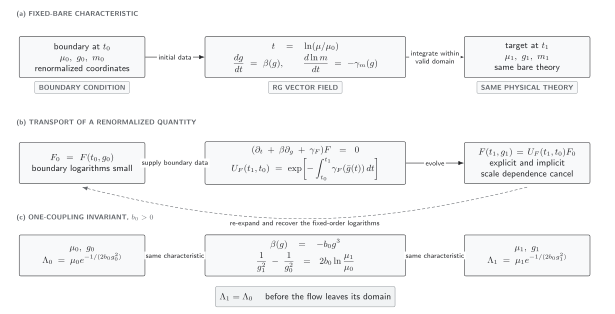
In panel (c), with gives , denoted above. Constancy is exact for this truncated vector field within its domain; the higher-order scale conventions are separate. is not the ultraviolet regulator cutoff. The diagram is schematic: approaching strong coupling indicates loss of perturbative control, not a plotted physical singularity.
| Figure element | Mathematical statement | Independent check |
|---|---|---|
| Characteristic through | with one boundary value | Differentiate the integrated solution and recover |
| Constant label on the curve | Substitute the running into | |
| Infrared end of the weak-coupling segment | is no longer large | Stop before the chosen perturbativity criterion fails |
What dimensional transmutation does—and does not—say
Section titled “What dimensional transmutation does—and does not—say”Consider a massless renormalized theory with one dimensionless coupling. The pair appears to contain a scale and a coupling, but changing while evolving along the same characteristic changes neither the bare theory nor a physical prediction. The invariant information can instead be written as the single dimensionful parameter :
within a declared scheme, coupling normalization, perturbative order, and flow branch. At one loop,
This is a one-to-one change of boundary coordinates, not an extra prediction. The exponential relation also creates a hierarchy:
when . Correspondingly,
at fixed and . Small changes in a weak reference coupling can therefore represent large multiplicative changes in the transmuted scale.
If a multiplicatively defined physical quantity has mass dimension , no other dimensional input, and no additive local ambiguity, RG invariance and dimensional analysis imply
or, with an external momentum ,
The dimensionless constant and the function need not be perturbatively calculable near . Perturbative running determines how the weak-coupling boundary datum is encoded in ; it does not generally determine a mass gap, bound-state spectrum, or confinement. When nonzero masses, relevant couplings, or thresholds are present, they supply additional invariant ratios and matching conditions.
This interpretation, including the fact that physical mass ratios are dimensionless constants while the common scale is transmuted, is developed in Collins 1984/2023, § 7.9, pp. 203–206.
Scheme and order labels
Section titled “Scheme and order labels”The numerical value of is not scheme independent. For a finite one-coupling redefinition
the first two beta-function coefficients are unchanged within mass-independent schemes, but the one-loop-normalized scales obey
That constant rescaling is not a physical contradiction. A matched dimensionless prediction, such as evaluated in the same scheme, transforms so that the observable is unchanged. The next page derives these finite-redefinition rules in detail.
A reproducible scale statement therefore has the form
| Required label | Example of what must be stated |
|---|---|
| Coupling definition | normalization of and the renormalized vertex or observable defining it |
| Subtraction scheme | for example, a declared mass-independent minimal-subtraction convention |
| Beta-function order | one term, two terms, or a higher declared truncation |
| Active degrees of freedom | particle content used in over the stated interval |
| Reference condition | or an equivalent matched value of |
| Validity and stopping rule | coupling bound, threshold, fixed point, or other event that terminates the evolution |
Analytic benchmark for RG-flow computation
Section titled “Analytic benchmark for RG-flow computation”A reproducible calculation begins with a one-coupling test whose exact answer is known. Its default equation and boundary data are
Thus
and the diagnostic invariant is
The exact reference values are:
A numerical solver should reproduce the invariant to relative tolerance , show on the positive branch, and reject evolution through . In a physical calculation the stronger stopping condition is normally reached earlier, when the coupling or the estimated omitted terms exceed the declared perturbative domain.
Regime limits and stopping events
Section titled “Regime limits and stopping events”An integrated RG trajectory is trustworthy only over the interval on which its inputs and approximation remain valid. Check the following events before interpreting the endpoint:
| Event | Why the current solution must stop or change | Correct continuation |
|---|---|---|
| becomes too large | Omitted beta-function terms are no longer demonstrably smaller | Switch to controlled nonperturbative information or report loss of control |
| A mass threshold is crossed | The active fields and beta coefficients change | Match onto the appropriate theory and continue with its beta function |
| reaches a reliable zero | The trajectory approaches a fixed point rather than a pole | Linearize about the zero and test stability and truncation dependence |
| A denominator in the truncated solution vanishes | The approximate ODE has left its weak-coupling branch | Do not continue through the formal singularity |
| A scheme map becomes singular or noninvertible | Coordinate equivalence has failed on that domain | Restrict to the invertible patch or choose a regular scheme |
| Large logarithms remain in the boundary calculation | Running alone did not choose all natural matching scales | Factorize or match at the relevant scales and evolve each object consistently |
The threshold problem is developed in Decoupling Theorems and Threshold Corrections. Fixed-point stability belongs to Fixed Points and Linearized RG Flow, and the systematic treatment of large logarithms appears later in this chapter.
Common pitfalls
Section titled “Common pitfalls”Calling scheme independent. It is RG invariant within a declared convention, but a finite coupling redefinition rescales it. Physical matched ratios are the invariant claims.
Equating a perturbative endpoint with a physical pole. A vanishing denominator says that the truncated weak-coupling solution has failed. It does not locate a pole of an exact observable.
Claiming that dimensional transmutation computes a mass gap. The RG converts into . A relation such as still contains dimensionless dynamics that may be nonperturbative.
Forgetting the flow branch. The integral of is branch dependent when beta functions have zeros or singularities. A boundary condition cannot be evolved through such a point by algebraic continuation alone.
Trusting an exact solution of a truncated beta function too far. Exact ODE integration removes numerical integration error; it does not remove perturbative truncation error.
Exercises
Section titled “Exercises”For , show directly that is invariant and derive the scale at which a trajectory with boundary value leaves the one-loop branch.
Solution
Differentiate along the flow:
The integrated solution is . Its denominator reaches zero at , hence . Perturbation theory must be stopped before that formal endpoint.
Let . Using only the one-loop definition of , derive the ratio .
Solution
The inverse coupling transforms as
Therefore, in the limit,
so . The finite factor must be included when translating any quantity quoted in units of .
Where to continue
Section titled “Where to continue”- Scheme Transformations and RG Invariants derives which beta-function data and fixed-point statements survive finite coordinate changes.
- Multiple Couplings and Coupled RG Flows replaces the one-dimensional trajectory by a vector field with stability matrices and separatrices.
- Large Logarithms and RG Improvement uses characteristic evolution to reorganize logarithmic perturbation theory.
References
Section titled “References”Original QFT.org content:CC BY 4.0, unless an item supplies different terms. Third-party material retains its own terms.