Power Counting and Predictive Order

A power counting is a rule that assigns an expected size to every operator insertion, loop, coupling, symmetry breaking, and observable contribution. Its practical output is an exhaustive list: at a requested accuracy, one can say which terms must be calculated and which first term is omitted. This page derives a homogeneous diagram formula, applies it to a scalar EFT with a dimension-six interaction, and shows how to detect a counting that is not closed.

Required background. Degrees of Freedom, Symmetry, and the Local Operator Expansion constructs the allowed interaction space. Scale Separation, Locality, and the Domain of an EFT fixes the expansion domain and hard scales. Helpful background. Asymptotic Scales, Remainders, Uniformity, and Optimal Truncation supplies the mathematical language for ordered remainders.

Predictive order is more than canonical dimension

Let $q=Q/\Lambda_b$ be a small kinematic ratio. An operator of dimension $d_i>4$ often enters with $q^{d_i-4}$, but this canonical estimate is only one ingredient. A complete counting can include

$$q, \qquad \frac{m_{\mathrm{light}}}{\Lambda_b}, \qquad \frac{g^2}{16\pi^2}, \qquad \varepsilon_{\mathrm{sym}}, \qquad \frac{Q}{4\pi f},$$

or other ratios appropriate to the system. A homogeneous counting assigns all of them powers of one bookkeeping parameter, or retains a transparent multigrading when their relative sizes are not fixed.

For example, declaring

$$\frac{Q^2}{\Lambda_b^2} \sim \frac{\lambda}{16\pi^2} \sim \varepsilon_{\mathrm{sym}} \sim q^2$$

means that a two-derivative higher-dimension insertion, one extra weak loop, and one insertion of the symmetry-breaking spurion contribute at the same relative order. The declaration is a physical assumption to test, not an identity.

Canonical dimension can fail as a ranking rule when:

• a symmetry forbids or suppresses a low-dimension operator;
• a small coupling or loop factor delays a contribution;
• a large occupation number or coherent background enhances it;
• anomalous dimensions substantially change scaling near a fixed point;
• a propagator becomes nearly on shell; or
• a shallow pole promotes repeated interactions.

The last case is treated separately on Nonperturbative Iteration, Shallow Scales, and Power-Counting Consistency. The ordinary perturbative derivation comes first.

Diagram scaling for a relativistic scalar EFT

Consider canonically normalized real scalars in four dimensions. Let a vertex of type $i$ contain $N_i$ fields and $D_i$ derivatives,

$$\mathcal L_i = \frac{c_i}{\Lambda_b^{d_i-4}} \partial^{D_i}\phi^{N_i}, \qquad d_i=D_i+N_i.$$

Numerical symmetry factors and index contractions are suppressed here; they belong to the operator definition. For a connected graph with $E$ external scalar legs, $I$ internal lines, $L$ loops, and $V_i$ vertices of type $i$, dimensional analysis gives

$$\mathcal A_E \sim \left(\frac{1}{16\pi^2}\right)^L Q^{4L-2I+\sum_iV_iD_i} \prod_i \frac{c_i^{V_i}}{\Lambda_b^{V_i(d_i-4)}}.$$

The graph identities are

$$L=I-\sum_iV_i+1, \qquad \sum_iV_iN_i=2I+E.$$

Substituting them into the power of $Q$ gives

$$4L-2I+\sum_iV_iD_i = 4-E+\sum_iV_i(d_i-4).$$

Therefore

$$\boxed{ \mathcal A_E \sim Q^{4-E} \left(\frac{1}{16\pi^2}\right)^L \prod_i \left[ c_i\left(\frac{Q}{\Lambda_b}\right)^{d_i-4} \right]^{V_i} }$$

for this declared weakly coupled scalar normalization. The overall $Q^{4-E}$ supplies the amplitude’s mass dimension. The relative EFT suppression is the product of higher-dimension insertions and loop factors.

If the bookkeeping assigns a vertex weight $\nu_i$ and one loop a weight $\nu_L$, the relative order is

$$\nu(\Gamma) = \sum_iV_i\nu_i+L\nu_L.$$

This compact formula is valid only after field normalization, propagator scaling, and all coupling weights have been fixed. Fermions, nonrelativistic propagators, medium modes, Goldstones, and gauge fields can change the topological reduction or the vertex assignments. Burgess derives the corresponding cutoff and dimensional-regularization counting logic in Burgess 2021, §§ 3.1–3.3, pp. 52–79.

Worked scalar example through relative order q²

Use two massless real scalars $\phi$ and $\chi$ with separate $\mathbb Z_2$ symmetries and

$$\mathcal L \supset -\frac{\lambda}{4}\phi^2\chi^2 +\frac{c_6}{2\Lambda_b^2} (\partial_\mu\phi)(\partial^\mu\phi)\chi^2.$$

The process $\phi\phi\to\chi\chi$ receives a momentum-independent tree amplitude from $\lambda$ and a dimension-six tree amplitude proportional to $c_6s/\Lambda_b^2$. Take

$$\begin{aligned} \frac{s}{\Lambda_b^2}&\sim q^2, &\frac{\lambda}{16\pi^2}&\sim q^2,\\ \lambda&\sim O(1), &\frac{c_6}{\lambda}&\sim O(1). \end{aligned}$$

Normalize the leading amplitude as $\mathcal A_{\mathrm{LO}}\sim\lambda$. Then the complete relative-$q^2$ contribution contains:

Contribution	Parametric size relative to $\mathcal A_{\mathrm{LO}}$	Why it is required
Tree insertion of the dimension-six operator	$c_6s/(\lambda\Lambda_b^2)$ under the declared coefficient normalization	First derivative correction
One-loop graphs built from leading marginal interactions	$\lambda/(16\pi^2)$	Same assigned order as $s/\Lambda_b^2$
Local counterterms for the one-loop divergences	Same order as the divergent loop structures	Regulator independence and closure
Renormalized-parameter and external-field corrections needed by the chosen observable	$q^2$ when generated by the same loops	Consistent input and LSZ normalization

The coefficient assumption needs care: if $\lambda$ is parametrically smaller than $c_6$, the ratio $c_6/\lambda$ changes the ordering. One may instead normalize the observable to a different reference amplitude or count $c_6$ with its own coupling suppression. The power counting must reflect the actual mechanism, not force every dimensionless coefficient to one.

At relative order $q^4$, the inventory generally adds dimension-eight trees, one-loop graphs with one relative-$q^2$ insertion, two-loop leading graphs, and all associated counterterms and parameter corrections. Whether a specific topology contributes can depend on field content and selection rules, but its absence must be demonstrated rather than assumed.

The diagram below summarizes the logic. A retained order is a complete vertical column, not a favorite subset of diagrams. The second panel previews how an infrared enhancement can promote an infinite subset without eliminating the need for counterterms or a first omitted order.

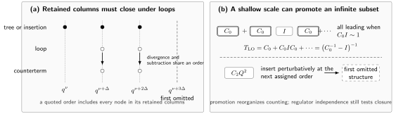
Predictive order requires closure. Panel (a) shows generic orders $q^\nu,q^{\nu+\Delta},\ldots$; each retained column must include every tree or insertion, loop, and local counterterm assigned to it, while the dashed column is the first omitted order. Panel (b) shows the distinct case $C_0I\sim1$, where a shallow scale promotes the entire $C_0$ iteration to leading order and higher-derivative structures remain perturbative. The diagram is schematic: $\Delta$ and the relative order of $C_2$ are theory dependent.

Loop factors and naive dimensional analysis

The explicit factor $1/(16\pi^2)^L$ is useful in a weakly coupled four-dimensional relativistic theory. It should not be applied mechanically. Strong dynamics can make the natural interaction scale closer to $4\pi f$ than to $f$, and a normalization that exposes this relation helps coefficients remain order one.

A common four-dimensional naive-dimensional-analysis form is

$$\mathcal L \sim \frac{\Lambda_b^4}{16\pi^2} \widehat{\mathcal L} \left( \frac{4\pi\phi}{\Lambda_b}, \frac{\partial}{\Lambda_b}, \frac{gA}{\Lambda_b}, \ldots \right).$$

Expanding $\widehat{\mathcal L}$ assigns correlated powers of $4\pi$ so that loops do not upset the assumed strong-coupling normalization. This is an estimate conditioned on the dynamics and field normalization, not a theorem that every coefficient lies between fixed numerical bounds.

If a coefficient is much larger or smaller than its estimate, ask whether:

• a symmetry, selection rule, or weak coupling explains the suppression;
• a nearby state or small denominator explains the enhancement;
• a field or operator normalization hid a power of $4\pi$;
• renormalization-group evolution produced a large logarithm; or
• the inferred $\Lambda_b$ is wrong.

Coefficient “naturalness” becomes a diagnostic only after these choices are visible.

Multiple expansions and anomalous scaling

Some problems have two genuinely independent small parameters, for example

$$q=\frac{Q}{\Lambda_b}, \qquad v\ll1.$$

There are three honest ways to proceed:

1. keep a bidegree $(n_q,n_v)$ and truncate a declared region of the lattice;
2. impose a relation such as $v\sim q$ when the physical regime justifies it; or
3. resum one hierarchy while expanding the other.

Silently replacing both by “small” makes the contribution inventory ambiguous. A term $q^2/v$ can dominate $q$ if $v\ll q$, and no canonical-dimension label reveals that.

Near a fixed point, an operator’s scaling dimension can be

$$\Delta_i = \Delta_i^{\mathrm{eng}}+\gamma_i^\star.$$

Its coupling then scales with the RG exponent $d-\Delta_i$, not merely its engineering dimension. For perturbative fixed points, $\gamma_i^\star$ can be included order by order. At strong coupling, importing canonical counting without nonperturbative scaling data can be qualitatively wrong. Relevant, Marginal, and Irrelevant Directions explains the RG classification; an EFT counting must still add kinematic and symmetry information specific to the observable.

A common uncertainty and validation checklist

Power counting defines only one part of the error budget. The following semantic record is reused through the remainder of the chapter so that a truncation estimate is never asked to cover unrelated errors.

Component	Record explicitly	Diagnostic or failure trigger
Domain and expansion parameters	Observable, kinematic window, $q_i(Q)$, hard scales, thresholds, and correlations among small parameters	A threshold enters, some $q_i\not\ll1$, or the assumed relation among parameters fails
Retained order and inventory	Highest order $k$, every tree, loop, insertion, counterterm, and parameter correction included	An omitted contribution has the same assigned order as a retained one
Coefficient assumptions	Operator normalization, scheme and scale, expected coefficient sizes, symmetry suppressions, and any priors	Coefficients drift with fit window or require unexplained enhancement
EFT truncation	First omitted powers, reference size, correlation model across energies and observables, and interval interpretation	Residuals do not scale with the predicted powers or coverage fails on withheld data
Input and fit uncertainty	Experimental or synthetic inputs, covariance, fitted combinations, and propagation method	Results are unstable under admissible input or fit-window changes
Numerical uncertainty	Solver, discretization, integration, rounding, convergence tolerance, and reproducibility data	Numerical changes are not parametrically below the claimed EFT error
Matching and running	Matching order and scale, anomalous dimensions, threshold sequence, and residual $\mu$ dependence	Scale cancellation fails through the retained order or a threshold is double counted
Regulator, basis, and scheme checks	Regulator range, required counterterms, field/basis map, and scheme transformation	Predictions depend on an auxiliary choice at or below the claimed order
Model discrepancy and breakdown	Effects not represented by the EFT, validation observables, stopping rule, and alternative field content	Persistent structured residuals, new nonanalyticity, or failure across observables

The record is a minimum schema, not a universal probability model. A deterministic remainder bound, a frequentist interval, and a Bayesian credible interval answer different questions and must be labeled accordingly.

Detecting inconsistent counting

A candidate counting fails before any numerical comparison if it violates one of these closure tests.

Equal-order omission. A tree correction is kept while a loop or parameter correction assigned the same $q$ power is dropped without a symmetry proof.

Missing counterterm. A retained loop generates a local divergence whose operator is absent or assigned to a later order. The operator must be included or the counting revised.

Hidden enhancement. A propagator, coefficient, or phase-space region carries inverse powers of a declared small parameter that were not included in the vertex weights.

Inhomogeneous subtraction. Different terms in the same physical prediction use incompatible field normalization, regulator, or renormalization scheme, so their stated orders cannot be compared.

Residual mismatch. After coefficients are fixed, the difference between successive orders or between EFT and reference data scales more slowly than the first omitted power.

A reproducible calculation uses the heavy-mediator residual to test the last condition and includes omitted-operator and double-counting cases. Loops, Counterterms, and Closure of an EFT Expansion develops the second condition explicitly.

Common pitfalls

Dimension determines order. Dimension supplies powers of the hard scale, while couplings, loops, symmetries, kinematics, and anomalous scaling determine the full hierarchy.

A loop is always one order higher. In some countings one loop costs $q^2$; in others it has a different weight, and in a promoted sector repeated loops are leading. Derive the loop scaling from measures and propagators.

Naive dimensional analysis predicts exact coefficient ranges. NDA is a normalization and conditional size estimate. It does not replace matching, data, or a mechanism-specific hierarchy.

The smallest visible correction is the uncertainty. An accidental zero can suppress one order. The first omitted contribution set and its correlations determine the truncation model.

Exercises

For the scalar graph formula, verify that a one-loop four-point graph with two dimension-four vertices has the correct mass dimension and no power of $Q/\Lambda_b$ beyond its loop factor.

Solution

Here $E=4$, $L=1$, and every vertex has $d_i-4=0$. The formula gives

$$\mathcal A_4 \sim Q^0\frac{c_4^2}{16\pi^2}.$$

A four-point amplitude is dimensionless in four dimensions. The loop is suppressed by $1/(16\pi^2)$ and couplings, but not by $Q/\Lambda_b$ because no higher-dimension insertion is present.

Assume $Q^2/\Lambda_b^2\sim\lambda/(16\pi^2)\sim q^2$. A calculation includes the dimension-six tree correction but omits the one-loop leading interaction. What accuracy can it consistently claim?

Solution

It cannot claim a complete relative-$q^2$ prediction, because the omitted loop is assigned exactly that order. At most it is a partial correction or a tree-level estimate. A complete claim requires the loop, its counterterms, and any same-order parameter or external-field corrections for the observable.

References

• Burgess, C. P. Introduction to Effective Field Theory: Thinking Effectively about Hierarchies of Scale. Cambridge: Cambridge University Press, 2021. DOI
• Weinberg, Steven. “Phenomenological Lagrangians.” Physica A: Statistical Mechanics and its Applications 96 (1979): 327–340. DOI