

Effective Average Actions and the Wetterich Equation
The effective average action is a scale-dependent 1PI generator constructed by adding an infrared quadratic kernel before taking a modified Legendre transform. For real bosons it obeys
The equation is exact because the inverse contains the full running Hessian. Its one-trace appearance does not make a finite ansatz exact. This page derives the sign, the inverse Hessian, the bosonic factor , the fermionic supertrace qualification, both endpoints, and a scalar local-potential projection whose one-loop coefficient can be checked analytically.
Required background. Wilsonian Coarse Graining and Theory Space supplies the physical scale interpretation and the exact-versus-projected distinction. The 1PI Effective Action and Mean-Field Equations supplies the ordinary Legendre transform, connected Hessian, and 1PI inverse-propagator relation.
Helpful background. The Polchinski Exact RG Equation develops the complementary Wilson-action formulation and fixes this chapter’s convention.
An infrared-regulated source functional
Section titled “An infrared-regulated source functional”For a real Euclidean bosonic field , add
to the microscopic action. With denoting integration over spacetime or momentum and contraction of internal indices, define
The average field and connected two-point function are
For a bosonic scalar, a useful regulator satisfies:
| Requirement | Operational meaning |
|---|---|
| for | Slow modes acquire an effective gap and do not yet fluctuate freely. |
| for | Modes well above are not distorted by the infrared regulator. |
| as | The ordinary unregulated generating functional is recovered at the infrared endpoint. |
| large at the starting scale | Fluctuations can be suppressed enough to match to declared microscopic data. |
| ultraviolet integrable | The trace is finite or is accompanied by an explicit ultraviolet regulator and renormalization prescription. |
Positivity is a bosonic stability condition, not a universal sign rule for every field species. Gauge fields, ghosts, and fermions require regulator matrices compatible with their quadratic forms and symmetry identities.
The modified Legendre transform
Section titled “The modified Legendre transform”Let solve . The effective average action is
Subtracting the regulator term is essential. Variation at fixed gives
Differentiate once more and use :
This is the exact inverse-Hessian identity. A zero eigenvalue of makes the flow singular, so the domain on which this operator is invertible is part of any existence or numerical claim.
Wetterich defines the infrared-regulated Legendre functional, proves this Hessian relation, and derives the exact scale equation in Wetterich 1993, pp. 90–94.
Deriving the exact trace
Section titled “Deriving the exact trace”Differentiate at fixed source:
At fixed , the terms containing cancel between and . Therefore
No loop expansion was used. The full depends on all vertices through . Replacing that Hessian by the Hessian of a finite polynomial, derivative expansion, or vertex ansatz is where approximation enters.
For a field multiplet, a compact convention is
The supertrace includes momentum and internal labels and inserts a minus sign for Grassmann-odd blocks. In a doubled fermionic field basis the displayed factor applies to the whole supermatrix. With an undoubled complex pair and regulator , the same content is conventionally written as a fermionic term without the bosonic half. The field ordering and doubling convention must accompany the formula.
The two exact-flow formulations
Section titled “The two exact-flow formulations”The figure reappears here to emphasize its right branch. Inspect the endpoint boxes: sending removes the modification from the Legendre transform, whereas sending in a Wilsonian representation does not turn its interaction action into .
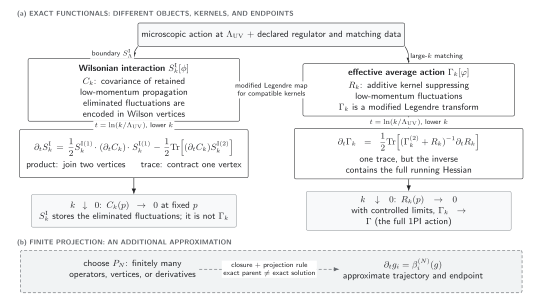
The solid branches are schematic exact identities for a regulated bosonic theory with . The effective average action uses an additive infrared kernel and tends to the ordinary 1PI action only when and the limit exists. A compatible modified Legendre map can relate it to a Wilsonian action, but the kernels, fields, boundary data, and endpoints remain distinct. The dashed layer marks the optional finite truncation, not part of either exact derivation.
| Item | Wilson interaction | Effective average action |
|---|---|---|
| Independent field | Retained integration field | Mean field |
| Scale kernel | Covariance | Additive inverse-propagator term |
| Exact flow structure | First-derivative product minus second-derivative trace | Full inverse-Hessian trace |
| Infrared statement | Wilson vertices encode eliminated fluctuations; no automatic 1PI endpoint | gives under controlled limits |
| Typical projection | Momentum-dependent Wilson vertices | Effective potential, derivative expansion, or 1PI vertices |
For complementary cutoff data, a generalized Legendre transform relates Wilsonian and infrared-regulated 1PI functionals Morris 1994, § 3, eqs. (3.25)–(3.28). This relation justifies the dotted cross-arrow; it does not identify the two boxes.
Ultraviolet matching and infrared endpoint
Section titled “Ultraviolet matching and infrared endpoint”If for every fixed as , then
provided the regulated functionals converge and the Legendre transform remains well defined. Under the usual positivity assumptions, the endpoint effective action has the convexity properties of a Legendre transform. A finite- potential need not yet be convex because is bounded together with rather than by itself.
At the opposite endpoint, a large positive suppresses fluctuations and makes a saddle approximation accurate. In an idealized limit this gives the field-dependent part of the microscopic action. In a theory initialized at a finite ultraviolet scale,
Thus is a boundary approximation whose accuracy depends on the ultraviolet cutoff, regulator, masses, and normalization. Wetterich states both the endpoint and the large- classical limit, including the finite-cutoff qualification, in Wetterich 1993, pp. 91–93.
Scalar local-potential flow
Section titled “Scalar local-potential flow”For one -symmetric scalar, take the local-potential ansatz
This ansatz fixes the wave-function coefficient to one and omits higher derivatives. At a constant field,
so the functional equation projects to
For an analytic evaluation, choose
Then ; the distribution from differentiating the step function is multiplied by and vanishes at its support. Define
The momentum integral is elementary:
The parent equation is exact, but this local-potential equation inherits the ansatz and regulator choice. The compact-support profile is convenient at this order; derivative projections require additional care at its nonsmooth boundary.
Expand
and set . Matching powers of gives
The running vacuum term is required for an absolute free energy. The quartic flow depends on , so a quartic polynomial is not an invariant subspace. Nevertheless, first affects the weak-coupling quartic beta function beyond . At , , and this order,
reproducing the shell and Polchinski checks.
A zero-dimensional exact benchmark
Section titled “A zero-dimensional exact benchmark”Zero dimensions remove momentum dependence without removing the Legendre transform or regulator logic. For
the trace has one entry and the exact equation is
For the Gaussian action , direct integration gives
Its derivative is exactly , matching the flow because . This checks the sign, factor , inverse Hessian, endpoint, and running vacuum contribution independently of a differential solver.
A reproducible calculation extends this benchmark to a quartic integral: exact quadrature is compared with matched polynomial flows, a running vacuum term, nested truncations, and more than one regulator. Zero dimensions do not test momentum or derivative expansions, but they sharply expose unmatched boundary data, Hessian singularities, and the mistake of calling a polynomial solution exact.
Checks and limitations
Section titled “Checks and limitations”- Regulator removal. Setting before differentiating makes and removes the flow; the endpoint is reached by integration followed by a controlled limit.
- Gaussian check. The zero-dimensional result verifies the complete normalization-sensitive equation, not only its field derivatives.
- One-loop check. The scalar local-potential projection reproduces in four dimensions with the declared coupling normalization.
- Exactness ceiling. The functional trace is exact, while the local-potential ansatz, polynomial expansion, regulator profile, and numerical solution are separate choices.
- Scope ceiling. The derivation is Euclidean and formal at the functional-integral level. Gauge identities, real-time contours, global existence, and subject-specific phenomenology require additional structures.
Common pitfalls
Section titled “Common pitfalls”Using the ordinary Legendre transform at finite . Omitting the subtraction changes the stationarity and Hessian identities. The flow then contains extra field-quadratic terms and is not the displayed Wetterich equation.
Reading “one trace” as “one loop only.” The line in the trace is the full field- and scale-dependent inverse Hessian. Expanding that inverse in microscopic couplings generates arbitrarily high perturbative loop orders.
Equating finite ultraviolet data with the classical action automatically. At a finite starting scale, regulator and cutoff corrections can remain. State how is matched and test the sensitivity to moving that scale.
Exercises
Section titled “Exercises”Derive from the modified Legendre transform.
Solution
Stationarity gives . Differentiating with respect to gives . Since , the two Jacobians are inverse operators, proving the identity.
For the compact-support regulator, derive the local-potential flow and the coefficient .
Solution
Inside , and . Outside, the numerator vanishes. Hence
The ball volume is , so the remaining factor is . Multiplying by gives the displayed result.
Show why omitting the vacuum term fails the zero-dimensional Gaussian benchmark.
Solution
The field-dependent Gaussian action has , so the exact right-hand side is the nonzero field-independent quantity . A truncation containing only has zero left-hand side at fixed and cannot satisfy the equation. Adding restores equality.
Continuations
Section titled “Continuations”- Functional-RG Truncations and Projection Methods turns the local-potential example into a controlled hierarchy of polynomial, grid, derivative, and vertex projections.
- Symmetry, Regulator Dependence, and Functional-RG Error Control develops modified identities, endpoint restoration, and a decomposed error statement.
- For a numerical check: compare the zero-dimensional flow against exact quadrature.
References
Section titled “References”Original QFT.org content:CC BY 4.0, unless an item supplies different terms. Third-party material retains its own terms.