

Wilsonian Coarse Graining and Theory Space
A Wilsonian effective action is the action for degrees of freedom that remain after a specified band of shorter-distance fluctuations has been integrated out. Because every symmetry-allowed interaction can be generated, changing resolution defines a trajectory in an infinite-dimensional theory space rather than merely changing the mass and one coupling of the starting Lagrangian.
This page defines that trajectory, performs a finite scalar shell integration far enough to display the induced operators, and separates exact blocking from rescaling and finite projection. The next page turns the same construction into differential mass and coupling flows near four dimensions.
Required background. Scale Independence and the Callan–Symanzik Equation supplies the contrasting fixed-bare flow. Gaussian Fields and Sources supplies the Gaussian functional integral used to eliminate a momentum sector.
Helpful background. Free-Field OPE Preview supplies the short-distance operator language that motivates a quasi-local expansion.
A Wilson action for the retained modes
Section titled “A Wilson action for the retained modes”Work in Euclidean signature with a real -symmetric scalar field and a finite ultraviolet cutoff . Begin with
Choose and split
where contains retained modes with and contains the eliminated band . The Wilson action is defined by
An overall normalization from the fast Gaussian determinant contributes to the vacuum term in . It cancels from normalized correlation functions but must be kept whenever a free energy or vacuum functional is the observable.
For sources supported below , this definition preserves the generating functional:
Nothing has yet been approximated. The cutoff, mode split, field measure, source support, and normalization are part of the definition. A sharp momentum shell makes the bookkeeping transparent; a smooth covariance is often preferable because it avoids nonanalytic dependence on a hard boundary in momentum space.
Wilson and Kogut formulate renormalization as successive reductions in the density of degrees of freedom followed by a comparison at restored resolution Wilson and Kogut 1974, § 1.1, pp. 78–83. Polchinski gives a smooth-cutoff QFT implementation in which lowering the cutoff changes an effective interaction while low-momentum correlation functions remain fixed Polchinski 1984, § 3, pp. 275–278.
Finite-shell scalar calculation
Section titled “Finite-shell scalar calculation”Let the fast Gaussian propagator be
where is one on the chosen shell and zero outside it for a sharp split. Write the fast Gaussian expectation as . Then
Define the shell moments
At first order,
Therefore
The interacting shell has already generated a vacuum shift and a mass shift:
At second order, take from each vertex the term
Since
its connected second cumulant gives
For external momenta small compared with , expand about . The leading local term is
so the unrescaled quartic coupling below the shell is
The sign refers to lowering the Wilsonian cutoff with and positive . It is compatible with a positive ultraviolet beta function after the flow direction and rescaling convention are translated.
The displayed terms do not close the action. Other connected contractions and higher cumulants generate
For the scalar example, momentum-dependent two-point terms begin at , while a local six-field term is generated at in the low-external-momentum expansion. The precise coefficients depend on the blocking kernel and projection. Their existence, not a universal finite coefficient, is the point of this page.
This is a quasi-local expansion: at fixed nonzero , the kernels can be expanded in external momenta divided by over a controlled domain. It is not a claim that the exact finite-shell functional is a finite polynomial in fields and derivatives. Thresholds, massless nonanalyticities, sharp cutoff surfaces, and external momenta comparable to can invalidate a derivative expansion.
Theory space, symmetry subspaces, and redundant directions
Section titled “Theory space, symmetry subspaces, and redundant directions”Write a quasi-local Wilson action as
The index ranges over vacuum terms, field monomials, derivative operators, tensor structures, and any other interactions allowed by the field content and regulator-compatible symmetries. Their coefficients are coordinates on an infinite-dimensional theory space.
Three distinct restrictions must not be conflated:
| Restriction | Meaning | Decisive test |
|---|---|---|
| Symmetry subspace | Operators forbidden by an exact preserved symmetry are excluded | The blocking measure and regulator preserve the symmetry, or a modified identity tracks its breaking |
| Quasi-local domain | Momentum kernels admit a derivative expansion around the declared external configuration | Higher derivative terms decrease over the claimed momentum range |
| Finite ansatz | Only a chosen list of coordinates is retained in a calculation | The exact flow’s components normal to are measured or bounded under systematic enlargement |
A field redefinition moves the coordinates without changing physical observables under the usual invertibility, Jacobian, source, and boundary assumptions. The tangent generated by such a redefinition is a redundant direction. It differs from a discarded normal component: the latter represents physical structures omitted by the ansatz, while the former is a change of description.
Wilson and Kogut explicitly describe the space of cutoff interactions as infinite dimensional, require it to contain the effective interactions generated by the transformation, and distinguish symmetry and canonical subspaces Wilson and Kogut 1974, § 12.1, pp. 159–163. The finite surface is therefore a convenient starting family, not an exact invariant subspace of scalar QFT.
Blocking, rescaling, and projection
Section titled “Blocking, rescaling, and projection”Let integrate the shell with . After blocking, the remaining cutoff is . To compare the new action with the old one at a fixed dimensionless cutoff, rescale
before any additional wavefunction normalization. Denote this rescaling by . One RG step is
The figure separates these operations and shows the geometric consequence of a finite ansatz. Inspect the normal projection from the exact action : it is distinct from the dotted field-redefinition direction.
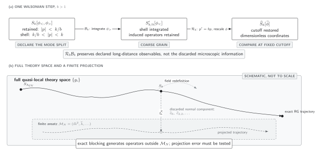
One Wilsonian step and its theory-space interpretation. For , modes with are integrated out before momenta and fields are rescaled; the exact quasi-local trajectory generally leaves the finite ansatz , so the projected trajectory requires an error test. The diagram is schematic and not to scale.
Without rescaling, disjoint shell integrations compose:
This follows directly by factorizing the Gaussian measure into the two disjoint shells. If the blocking and normalization prescriptions are self-similar, the rescaled maps obey
Physical coarse graining forms a semigroup: integration discards microscopic information, so a generic blocked action does not determine a unique microscopic action. A differential flow may be integrated backward locally on a restricted image, but that mathematical operation is not a general inverse to coarse graining. Wilson and Kogut analyze the nested images and topology of the transformation in Wilson and Kogut 1974, § 12.1, pp. 159–166.
Dimensionless coordinates
Section titled “Dimensionless coordinates”Let have canonical dimension and let multiply . Define
Using the infrared-directed variable
the canonical part of the flow is
For the scalar kinetic normalization used above,
The rescaling step is what exposes this canonical competition with fluctuations. A dimensionful coupling can decrease while its dimensionless coordinate grows, or vice versa. Fixed-point eigenvalues and the labels relevant, marginal, and irrelevant require linearization about a specified fixed point and a declared RG direction; they are developed in Fixed Points, Universality, and Continuum Limits.
Four scale operations compared
Section titled “Four scale operations compared”| Operation | Scale varied | What changes | What is preserved or tested |
|---|---|---|---|
| Regulator removal | Auxiliary or | Regulated intermediate expressions and counterterms | Renormalized observables have a removal limit |
| Callan–Symanzik running | Subtraction scale | Renormalized parameters and field normalizations | The complete prediction is independent |
| Wilsonian blocking | Resolution scale | The action for retained modes | Long-distance generating functionals agree after matching sources and normalization |
| Effective-average-action flow | Infrared suppression scale | The regulated 1PI functional | The exact modified Legendre construction connects matched initial data to |
The same symbol can appear in several roles in the literature. The operation, not the letter, determines the meaning.
Checks and limitations
Section titled “Checks and limitations”A defensible coarse-graining statement records:
- the cutoff shape and whether it is sharp or smooth;
- the exact fast and retained mode domains;
- the source support and observable preserved by blocking;
- the vacuum normalization;
- the coordinate and field rescaling;
- the symmetry subspace and any modified identity;
- the quasi-local expansion parameter ;
- every projected-away operator class; and
- an enlargement or independent benchmark for the truncation.
This page gives a perturbative Euclidean scalar construction. It does not establish a nonperturbative continuum measure, positivity after an arbitrary momentum cutoff, convergence of the derivative expansion, or the existence of a fixed point. Rigorous RG as a Dynamical System and Renormalized Trajectories and Counterterm Tuning develop theorem-level versions under explicit hypotheses.
Common pitfalls
Section titled “Common pitfalls”Keeping only the couplings present in the microscopic action. Shell contractions generate every structure allowed by the symmetries and kinematics. A two-coupling calculation is a projection whose discarded components must be tested.
Calling a sharp cutoff local. A Wilson action can be quasi-local for external momenta well below , but a sharp boundary produces nonanalytic momentum dependence near the shell. State the domain of the derivative expansion.
Confusing blocking with rescaling. Integration lowers the remaining cutoff; rescaling restores a common dimensionless cutoff for comparison. Canonical scaling enters only after the second operation.
Treating coarse graining as invertible. The maps compose, but eliminated microscopic information is not generically recoverable. A backward solution of a differential equation exists only on a restricted trajectory and with additional data.
Calling every field-coordinate motion physical. Redundant directions generated by admissible field redefinitions must be quotiented before interpreting a projected coupling as an observable.
Exercises
Section titled “Exercises”Derive the one-shell mass and quartic shifts.
Solution
The first cumulant contains
Matching the quadratic term to gives
For the quartic term, the connected contraction of two vertices is
At leading order in external momenta this is
Since the quartic normalization is , the shift is
Prove the composition law for two unrescaled shell integrations.
Solution
Split
The Gaussian measure factorizes over the two disjoint fast sectors. Integrating the upper shell first gives ; integrating the next shell gives . Fubini’s theorem for the finite regulated integral permits the order to be combined:
Thus
including the accumulated vacuum normalization.
Continuations
Section titled “Continuations”- Momentum-Shell Integration and Rescaling takes the thin-shell limit and derives dimensionless scalar mass and quartic flows near four dimensions.
- The Polchinski Exact RG Equation derives a smooth-cutoff differential equation for the full Wilson interaction action.
- Effective Average Actions and the Wetterich Equation develops the distinct scale-dependent 1PI functional.
- Stable Manifolds and Relevant–Marginal Control supplies the theorem-level geometry behind controlled trajectory statements.
References
Section titled “References”Original QFT.org content:CC BY 4.0, unless an item supplies different terms. Third-party material retains its own terms.